Numerical solution methods - Essential Mathematics for Chemical Engineers

Systems of first-order ODEs can also be solved numerically using similar approaches as for single first-order ODEs, but now all dependent variables must be advanced simultaneously. The methods we use for single first-order ODES can be straightforwardly extended to systems using the explicit-form vector notation $\vv{y}' = \vv{f}(t, \vv{y})$ . For example, Euler’s method becomes:

\vv{y}(t+\Delta t) \approx \vv{y}(t) + \vv{f}(t, \vv{y}) \Delta t

(1)

We are “just” adding columns to our calculations!

Example: First-order reaction in a draining tank¶

A first-order reaction (rate constant k) is taking place in a tank that is initially 1 M concentration in the reactant A and has 10 L of solution. A feed stream that has a reactant concentration of 1 M enters at 1 L / min, while well-mixed solution exits at 2 L / min.

$Reactions in draining tank.$

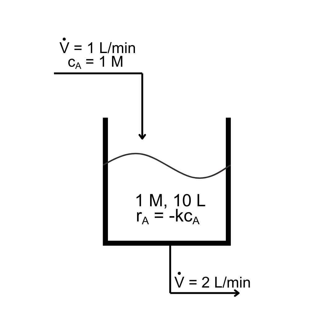
Estimate the concentration of A after 1 minute if $k = 0.5/{\rm min}$ .

Start from an unsteady mole balance on A:

\dd{}{n_{\rm A}}{t} = \dot n_{{\rm A},{\rm in}} - \dot n_{{\rm A},{\rm out}} + r_A V

(2)

The number of moles in the tank, the molar flow rate in, and the molar flow rate out are:

\begin{align} n_{\rm A} &= c_{\rm A} V \\ \dot n_{{\rm A},{\rm in}} &= c_{{\rm A},{\rm in}} \dot V_{\rm in} = 1 \\ \dot n_{{\rm A},{\rm out}} &= c_{\rm A} \dot V_{\rm out} = 2c_A \end{align}

(3)

\begin{align} \dd{}{(Vc_{\rm A})}{t} &= 1 - 2 c_A - k c_A V \\ V \dd{}{c_{\rm A}}{t} + c_{\rm A} \dd{}{V}{t} &= 1 - 2 c_A - k c_A V \end{align}

(4)

Since the volume V is changing, write a mass balance on the tank assuming that the solution density $\rho$ does not depend on concentration:

\begin{align} \dd{}{m}{t} = \dot m_{\rm in} - \dot m_{\rm out} \end{align}

(5)

with the mass in the tank, mass flow rate in, and mass flow rate out:

\begin{align} m &= \rho V \\ \dot m_{\rm in} &= \rho \dot V_{\rm in} = \rho \\ \dot m_{\rm out} &= \rho \dot V_{\rm out} = 2 \rho \end{align}

(6)

\begin{align} \dd{}{(V\rho)}{t} = \rho \dd{}{V}{t} &= -\rho \\ \dd{}{V}{t} &= - 1 \end{align}

(7)

Substituting for $\dd{}{V}{t}$ in the unsteady mole balance and rearranging gives the system of first-order ODES:

\begin{align} \dd{}{c_{\rm A}}{t} &= \frac{1}{V} \left(1 - c_A - 0.5Vc_A\right),& c_{\rm A}(0) &= 1 \\ \dd{}{V}{t} &= -1, & V(0) &= 10 \end{align}

(8)

Calling $y_1 = c_{\rm A}$ and $y_2 = V$ :

$n$	$t$	$y_1$	$y_2$	$f_1$	$f_2$
0	0	1	10	-0.5	-1
1	0.2	0.9	9.8	-0.4398	-1
2	0.4	0.8120	9.6	-0.3864	-1
3	0.6	0.7347	9.4	-0.3389	-1
4	0.8	0.6669	9.2	-0.2972	-1
5	1.0	.6075	9

The concentration after 1 minute is approximately 0.6 M.

Skill builder problems¶

Solution to Exercise 1

The ODE is already in explicit form, so start solving from the initial condition.

$n$	$t$	$y_1$	$y_2$	$f_1$	$f_2$
0	0	1.500	1.000	-1.000	0.500
1	0.5	1.000	1.250	-1.000	0.000
2	1.0	0.500	1.250	-0.500	-0.625
3	1.5	0.250	0.938	-0.146	-0.703
4	2.0	0.177	0.586	-0.020	-0.482
5	2.5	0.167	0.345	0.035	-0.287
6	3.0	0.184	0.201	0.073	-0.164
7	3.5	0.221	0.120	0.112	-0.093
8	4.0	0.277	0.073	0.158	-0.053
9	4.5	0.356	0.046	0.215	-0.030
10	5.0	0.464	0.032

The final result is $y_1(5) = 0.464$ and $y_2(5) = 0.032$ .

6.4 Numerical solution methods

Example: First-order reaction in a draining tank¶

Skill builder problems¶