6.3 Homogeneous linear first-order ODEs with constant coefficients
Systems of homogeneous linear first-order ODEs with constant coefficients can
be written in the form:
y ′ = A y \vv{y}' = \vv{A} \vv{y} y ′ = Ay Let’s guess a solution of the form:
y = e λ t x y ′ = λ e λ t x \begin{align}
\vv{y} &= e^{\lambda t} \vv{x} \\
\vv{y}' &= \lambda e^{\lambda t} \vv{x}
\end{align} y y ′ = e λ t x = λ e λ t x Substituting in the ODE:
λ e λ t x = A e λ t λ x = A x \begin{align}
\lambda e^{\lambda t} \vv{x} &= \vv{A} e^{\lambda t}\\
\lambda \vv{x} &= \vv{A} \vv{x}
\end{align} λ e λ t x λ x = A e λ t = Ax We find that our solution must satisfy an eigenvalue problem! λ \lambda λ x is an eigenvector of A . We know an n x n matrix
has n eigenvalues. Let’s suppose the corresponding eigenvectors are all
linearly independent. What do we do?
In practice, this means that
y = ∑ i = 1 n c i e λ i t x i = c 1 e λ 1 t x 1 + ⋯ + c n e λ n t x n \vv{y} = \sum_{i=1}^n c_i e^{\lambda_i t} \vv{x}_i
= c_1 e^{\lambda_1 t}\vv{x}_1 + \cdots + c_n e^{\lambda_n t}\vv{x}_n y = i = 1 ∑ n c i e λ i t x i = c 1 e λ 1 t x 1 + ⋯ + c n e λ n t x n (There are some cases this fails, but we will not cover them.) To apply the
initial condition y ( 0 ) = y 0 \vv{y}(0) = \vv{y}_0 y ( 0 ) = y 0
y ( 0 ) = c 1 x 1 + ⋯ c n x n = y 0 X c = y 0 \begin{align}
\vv{y}(0) = c_1 \vv{x}_1 + \cdots c_n \vv{x}_n &= \vv{y}_0 \\
\vv{X} \vv{c} &= \vv{y}_0
\end{align} y ( 0 ) = c 1 x 1 + ⋯ c n x n Xc = y 0 = y 0 where X = [ x 1 ⋯ x n ] \vv{X} = [\vv{x}_1 \cdots \vv{x}_n] X = [ x 1 ⋯ x n ] A and c is the column vector of unknown coefficients.
Example: Reaction network (again) ¶ We previously analyzed the concentration of three species (A, B, and C)
undergoing a sequence of first-order reactions, A → B → C A \to B \to C A → B → C k 1 k_1 k 1 k 2 k_2 k 2
c ′ = A c , c ( 0 ) = [ c A , 0 0 0 ] \vv{c}' = \vv{A} \vv{c}, \quad
\vv{c}(0) = \begin{bmatrix} c_{{\rm A},0} \\ 0 \\ 0 \end{bmatrix} c ′ = Ac , c ( 0 ) = ⎣ ⎡ c A , 0 0 0 ⎦ ⎤ where
c = [ c A c B c C ] A = [ − k 1 0 0 k 1 − k 2 0 0 k 2 0 ] \vv{c} = \begin{bmatrix} c_{\rm A} \\ c_{\rm B} \\ c_{\rm C} \end{bmatrix} \qquad
\vv{A} = \begin{bmatrix} -k_1 & 0 & 0 \\ k_1 & -k_2 & 0 \\ 0 & k_2 & 0 \end{bmatrix} c = ⎣ ⎡ c A c B c C ⎦ ⎤ A = ⎣ ⎡ − k 1 k 1 0 0 − k 2 k 2 0 0 0 ⎦ ⎤ Solve again using eigenvalues and eigenvectors.
A is lower triangular, so its eigenvalues are: λ 1 = − k 1 \lambda_1 = -k_1 λ 1 = − k 1 λ 2 = − k 2 \lambda_2 = -k_2 λ 2 = − k 2 λ 3 = 0 \lambda_3 = 0 λ 3 = 0 λ 1 = − k 1 \lambda_1 = -k_1 λ 1 = − k 1
A − λ 1 I = [ 0 0 0 k 1 − k 2 + k 1 0 0 k 2 k 1 ] \vv{A} - \lambda_1 \vv{I} =
\begin{bmatrix} 0 & 0 & 0 \\ k_1 & -k_2 + k_1 & 0 \\ 0 & k_2 & k_1 \end{bmatrix} A − λ 1 I = ⎣ ⎡ 0 k 1 0 0 − k 2 + k 1 k 2 0 0 k 1 ⎦ ⎤ from which we obtain two equations:
k 1 x 1 − ( k 2 − k 1 ) x 2 = 0 k 2 x 2 + k 1 x 3 = 0 \begin{align}
k_1 x_1 - (k_2 - k_1) x_2 &= 0 \\
k_2 x_2 + k_1 x_3 &= 0 \\
\end{align} k 1 x 1 − ( k 2 − k 1 ) x 2 k 2 x 2 + k 1 x 3 = 0 = 0 with x 3 x_3 x 3 x 3 = 1 x_3 = 1 x 3 = 1
x 1 = [ − k 2 − k 1 k 2 − k 1 k 2 1 ] \vv{x}_1 = \begin{bmatrix} \dfrac{-k_2 - k_1}{k_2} \\ \dfrac{-k_1}{k_2} \\ 1 \end{bmatrix} x 1 = ⎣ ⎡ k 2 − k 2 − k 1 k 2 − k 1 1 ⎦ ⎤ Next, we will solve with λ 2 = − k 2 \lambda_2 = -k_2 λ 2 = − k 2
A − λ 2 I = [ k 2 − k 1 0 0 k 1 0 0 0 k 2 k 2 ] \vv{A} - \lambda_2 \vv{I} =
\begin{bmatrix} k_2-k_1 & 0 & 0 \\ k_1 & 0 & 0 \\ 0 & k_2 & k_2 \end{bmatrix} A − λ 2 I = ⎣ ⎡ k 2 − k 1 k 1 0 0 0 k 2 0 0 k 2 ⎦ ⎤ from which we obtain:
x 2 = [ 0 − 1 1 ] \vv{x}_2 = \begin{bmatrix} 0 \\
-1 \\
1 \end{bmatrix} x 2 = ⎣ ⎡ 0 − 1 1 ⎦ ⎤ Finally, we solve with λ 3 = 0 \lambda_3 = 0 λ 3 = 0
A − λ 3 I = [ − k 1 0 0 k 1 − k 2 0 0 k 2 0 ] \vv{A} - \lambda_3 \vv{I} =
\begin{bmatrix} -k_1 & 0 & 0 \\ k_1 & -k_2 & 0 \\ 0 & k_2 & 0 \end{bmatrix} A − λ 3 I = ⎣ ⎡ − k 1 k 1 0 0 − k 2 k 2 0 0 0 ⎦ ⎤ from which we obtain:
x 3 = [ 0 0 1 ] \vv{x}_3 = \begin{bmatrix} 0\\
0 \\
1 \end{bmatrix} x 3 = ⎣ ⎡ 0 0 1 ⎦ ⎤ Hence, the general solution is
c = a 1 e − k 1 t [ − k 2 − k 1 k 2 − k 1 k 2 1 ] + a 2 e − k 2 t [ 0 − 1 1 ] + a 3 e 0 t [ 0 0 1 ] \vv{c} = a_1 e^{-k_1t} \begin{bmatrix}
\dfrac{-k_2 - k_1}{k_2} \\ \dfrac{-k_1}{k_2} \\ 1 \end{bmatrix} +
a_2 e^{-k_2t} \begin{bmatrix} 0 \\ -1 \\ 1 \end{bmatrix} +
a_3 e^{0 t} \begin{bmatrix} 0\\ 0 \\ 1 \end{bmatrix} c = a 1 e − k 1 t ⎣ ⎡ k 2 − k 2 − k 1 k 2 − k 1 1 ⎦ ⎤ + a 2 e − k 2 t ⎣ ⎡ 0 − 1 1 ⎦ ⎤ + a 3 e 0 t ⎣ ⎡ 0 0 1 ⎦ ⎤ Now, we apply the initial condition:
[ − k 2 − k 1 k 2 0 0 − k 1 k 2 − 1 0 1 1 1 ] [ a 1 a 2 a 3 ] = [ c A , 0 0 0 ] \begin{align}
\begin{bmatrix}
\dfrac{-k_2 - k_1}{k_2} & 0 & 0 \\
\dfrac{-k_1}{k_2} & -1 & 0 \\
1 & 1 & 1
\end{bmatrix}
\begin{bmatrix}
a_1 \\ a_2 \\ a_3
\end{bmatrix} =
\begin{bmatrix} c_{{\rm A},0}\\ 0 \\ 0 \end{bmatrix}
\end{align} ⎣ ⎡ k 2 − k 2 − k 1 k 2 − k 1 1 0 − 1 1 0 0 1 ⎦ ⎤ ⎣ ⎡ a 1 a 2 a 3 ⎦ ⎤ = ⎣ ⎡ c A , 0 0 0 ⎦ ⎤ Thus,
a 1 = − c A , 0 k 2 k 2 − k 1 a 2 = − k 1 k 2 a 1 = c A , 0 k 1 k 2 − k 1 a 3 = − a 1 − a 2 = c A , 0 \begin{align}
a_1 &= -c_{{\rm A},0}\frac{k_2}{k_2-k_1} \\
a_2 &= -\frac{k_1}{k_2}a_1 = c_{{\rm A},0}\frac{k_1}{k_2-k_1} \\
a_3 &= -a_1 - a_2 = c_{{\rm A},0}
\end{align} a 1 a 2 a 3 = − c A , 0 k 2 − k 1 k 2 = − k 2 k 1 a 1 = c A , 0 k 2 − k 1 k 1 = − a 1 − a 2 = c A , 0 Finally, substitute these constants into the general solution and add across
the rows to obtain solutions for each concentration:
c A ( t ) = a 1 e − k 1 t − k 2 − k 1 k 2 = c A , 0 e − k 1 t c B ( t ) = a 1 e − k 1 t − k 1 k 2 − a 2 e − k 2 t = c A , 0 k 1 k 2 − k 1 ( e − k 1 t − e − k 2 t ) c C ( t ) = a 1 e − k 1 t + a 2 e − k 2 t + a 3 = c A , 0 ( 1 − k 2 k 2 − k 1 e − k 1 t + k 1 k 2 − k 1 e − k 2 t ) \begin{align}
c_{\rm A}(t) &= a_1e^{-k_1t}\frac{-k_2-k_1}{k_2} = c_{{\rm A},0}e^{-k_1t} \\
c_{\rm B}(t) &= a_1e^{-k_1t}\frac{-k_1}{k_2} - a_2e^{-k_2t} \\
&= c_{{\rm A},0}\frac{k_1}{k_2 - k_1}(e^{-k_1t} - e^{-k_2t}) \\
c_{\rm C}(t) &= a_1e^{-k_1t} + a_2e^{-k_2t} + a_3 \\
&= c_{{\rm A},0}\Biggl(1 - \frac{k_2}{k_2 - k_1} e^{-k_1t} +
\frac{k_1}{k_2 - k_1} e^{-k_2t}\Biggr)
\end{align} c A ( t ) c B ( t ) c C ( t ) = a 1 e − k 1 t k 2 − k 2 − k 1 = c A , 0 e − k 1 t = a 1 e − k 1 t k 2 − k 1 − a 2 e − k 2 t = c A , 0 k 2 − k 1 k 1 ( e − k 1 t − e − k 2 t ) = a 1 e − k 1 t + a 2 e − k 2 t + a 3 = c A , 0 ( 1 − k 2 − k 1 k 2 e − k 1 t + k 2 − k 1 k 1 e − k 2 t ) This matches our old answer!
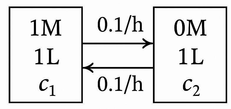
Example: Diffusion cell ¶ Consider a diffusion cell consisting of two compartments with solute
concentrations c 1 c_1 c 1 c 2 c_2 c 2
Based on unsteady mole balances, the concentrations change according to:
c 1 ′ = − 0.1 c 1 + 0.1 c 2 c 2 ′ = 0.1 c 1 − 0.1 c 2 \begin{align}
c_1' &= -0.1c_1 + 0.1c_2 \\
c_2' &= 0.1c_1 - 0.1c_2
\end{align} c 1 ′ c 2 ′ = − 0.1 c 1 + 0.1 c 2 = 0.1 c 1 − 0.1 c 2 Solve for c 1 c_1 c 1 c 2 c_2 c 2
Write in matrix form c ′ = A c \vv{c}' = \vv{A} \vv{c} c ′ = Ac
c = [ c 1 c 2 ] A = [ − 0.1 0.1 0.1 − 0.1 ] \vv{c} = \begin{bmatrix}c_1 \\ c_2\end{bmatrix}
\qquad \vv{A} = \begin{bmatrix} -0.1 & 0.1 \\ 0.1 & -0.1 \end{bmatrix} c = [ c 1 c 2 ] A = [ − 0.1 0.1 0.1 − 0.1 ] Since A is symmetric, it has real eigenvalues:
∣ A − λ I ∣ = ∣ − 0.1 − λ 0.1 0.1 − 0.1 − λ ∣ = ( λ + 0.1 ) 2 − 0. 1 2 = λ 2 + 0.2 λ = λ ( λ + 0.2 ) = 0 \begin{align}
|\vv{A} - \lambda \vv{I}|
&= \begin{vmatrix} -0.1 - \lambda & 0.1 \\ 0.1 & -0.1 - \lambda \end{vmatrix}\\
&= (\lambda + 0.1)^2 - 0.1^2 \\
&= \lambda^2 + 0.2\lambda \\
& = \lambda(\lambda + 0.2) = 0
\end{align} ∣ A − λ I ∣ = ∣ ∣ − 0.1 − λ 0.1 0.1 − 0.1 − λ ∣ ∣ = ( λ + 0.1 ) 2 − 0. 1 2 = λ 2 + 0.2 λ = λ ( λ + 0.2 ) = 0 So, the eigenvalues are λ 1 = 0 \lambda_1 = 0 λ 1 = 0 λ 2 = − 0.2 \lambda_2 = -0.2 λ 2 = − 0.2
A − λ 1 I = [ − 0.1 0.1 0.1 − 0.1 ] → x 1 = [ 1 1 ] A − λ 2 I = [ 0.1 0.1 0.1 0.1 ] → x 2 = [ 1 − 1 ] \begin{align}
\vv{A}-\lambda_1 \vv{I} &= \begin{bmatrix} -0.1 & 0.1 \\ 0.1 & -0.1 \end{bmatrix}
\to \vv{x}_1 = \begin{bmatrix} 1 \\ 1 \end{bmatrix} \\
\vv{A} - \lambda_2 \vv{I} &= \begin{bmatrix} 0.1 & 0.1 \\ 0.1 & 0.1 \end{bmatrix}
\to \vv{x}_2 = \begin{bmatrix} 1 \\ -1 \end{bmatrix}
\end{align} A − λ 1 I A − λ 2 I = [ − 0.1 0.1 0.1 − 0.1 ] → x 1 = [ 1 1 ] = [ 0.1 0.1 0.1 0.1 ] → x 2 = [ 1 − 1 ] The general solution is:
c ( t ) = a 1 e 0 t [ 1 1 ] + a 2 e − 0.2 t [ 1 − 1 ] = a 1 [ 1 1 ] + a 2 e − 0.2 t [ 1 − 1 ] \begin{align}
\vv{c}(t) &= a_1 e^{0t} \begin{bmatrix} 1 \\ 1 \end{bmatrix} +
a_2 e^{-0.2t} \begin{bmatrix} 1 \\ -1 \end{bmatrix} \\
&= a_1 \begin{bmatrix} 1 \\ 1 \end{bmatrix} + a_2 e^{-0.2t}
\begin{bmatrix} 1 \\ -1 \end{bmatrix}
\end{align} c ( t ) = a 1 e 0 t [ 1 1 ] + a 2 e − 0.2 t [ 1 − 1 ] = a 1 [ 1 1 ] + a 2 e − 0.2 t [ 1 − 1 ] Apply the initial conditions by solving X a = c ( 0 ) \vv{X}\vv{a} = \vv{c}(0) Xa = c ( 0 )
[ 1 1 1 1 − 1 0 ] R 1 − R 1 → [ 1 1 1 0 − 2 − 1 ] R 1 ÷ − 2 → [ 1 1 1 0 1 1 / 2 ] − R 2 R 2 → [ 1 0 1 / 2 0 1 1 / 2 ] \begin{align}
\begin{bmatrix} 1 & 1 & 1\\ 1 & -1 & 0\end{bmatrix}
\begin{matrix}\vphantom{R_1} \\ -R_1 \end{matrix}
&\to \begin{bmatrix} 1 & 1 & 1\\ 0 & -2 & -1\end{bmatrix}
\begin{matrix}\vphantom{R_1} \\ \div -2 \end{matrix} \\
&\to \begin{bmatrix} 1 & 1 & 1\\ 0 & 1 & 1/2\end{bmatrix}
\begin{matrix} -R_2 \\ \vphantom{R_2} \end{matrix} \\
&\to \begin{bmatrix} 1 & 0 & 1/2 \\ 0 & 1 & 1/2\end{bmatrix}
\end{align} [ 1 1 1 − 1 1 0 ] R 1 − R 1 → [ 1 0 1 − 2 1 − 1 ] R 1 ÷ − 2 → [ 1 0 1 1 1 1/2 ] − R 2 R 2 → [ 1 0 0 1 1/2 1/2 ] so a 1 = a 2 = 1 / 2 a_1 = a_2 = 1/2 a 1 = a 2 = 1/2 c ( t ) \vv{c}(t) c ( t )
c ( t ) = 1 2 [ 1 1 ] + 1 2 e − 0.2 t [ 1 − 1 ] \vv{c}(t) = \frac{1}{2} \begin{bmatrix} 1 \\ 1 \end{bmatrix} +
\frac{1}{2} e^{-0.2t} \begin{bmatrix} 1 \\ -1 \end{bmatrix} c ( t ) = 2 1 [ 1 1 ] + 2 1 e − 0.2 t [ 1 − 1 ] or equivalently
c 1 ( t ) = 1 2 ( 1 + e − 0.2 t ) c 2 ( t ) = 1 2 ( 1 − e − 0.2 t ) \begin{align}
c_1(t) &= \frac{1}{2} \left(1 + e^{-0.2 t}\right) \\
c_2(t) &= \frac{1}{2} \left(1 - e^{-0.2 t}\right)
\end{align} c 1 ( t ) c 2 ( t ) = 2 1 ( 1 + e − 0.2 t ) = 2 1 ( 1 − e − 0.2 t ) Types of critical points ¶ We can use the eigenvalues and eigenvectors to anticipate what solutions
around critical points (y ′ = 0 \vv{y}' = \vv{0} y ′ = 0
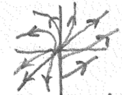
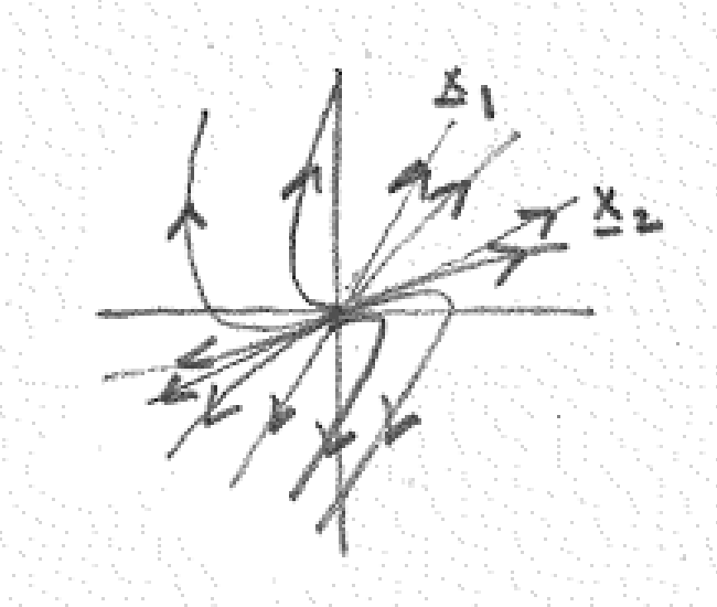
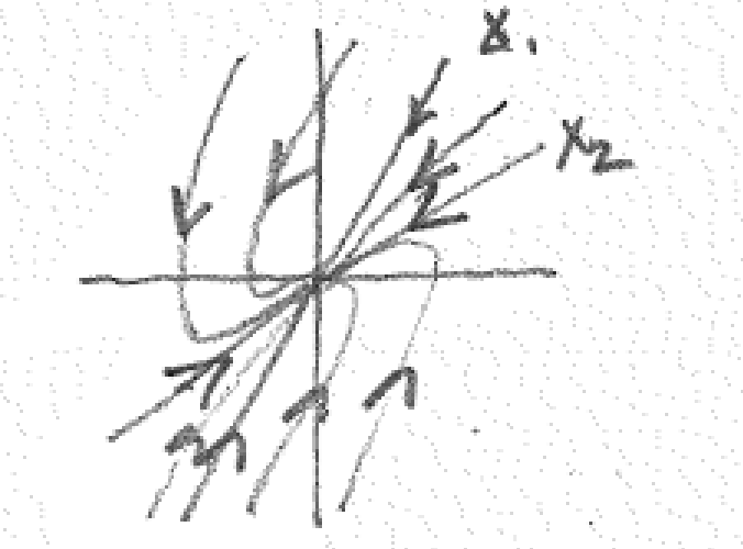
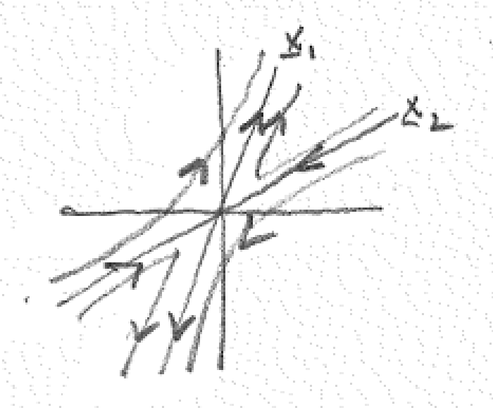
If the eigenvalues are real and distinct, λ 1 ≠ λ 2 \lambda_1 \ne \lambda_2 λ 1 = λ 2
Unstable improper node
λ 1 > λ 2 > 0 \lambda_1 > \lambda_2 > 0 λ 1 > λ 2 > 0 Stable improper node
λ 1 < λ 2 < 0 \lambda_1 < \lambda_2 < 0 λ 1 < λ 2 < 0 Saddle
λ 1 > 0 , λ 2 < 0 \lambda_1 > 0, \quad \lambda_2 < 0 λ 1 > 0 , λ 2 < 0 If the eigenvalues are complex, λ 1 , 2 = α ± i ω \lambda_{1,2} = \alpha \pm i\omega λ 1 , 2 = α ± iω
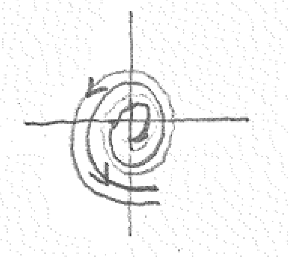
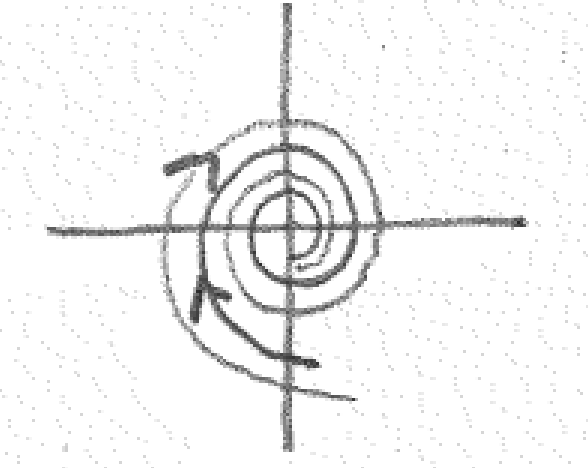
Unstable spiral
Stable spiral
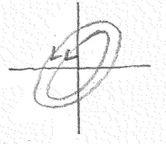
Center
The direction of the orbit depends on the matrix and can be checked for
some point. If
A = [ a b c d ] \vv{A} = \begin{bmatrix}a & b \\ c & d\end{bmatrix} A = [ a c b d ] The orbit is clockwise if b > c b > c b > c c < b c < b c < b
If the eigenvalues are real and repeated, λ 1 = λ 2 \lambda_1 = \lambda_2 λ 1 = λ 2
Proper node / star
A is a multiple of I .
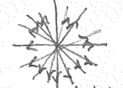
Degenerate node
Skill builder problems ¶ Solve the inital value problem y ′ = A y \vv{y}' = \vv{A}\vv{y} y ′ = Ay y ( 0 ) = [ 1 0 ] T \vv{y}(0) = [1 \quad 0]^{\rm T} y ( 0 ) = [ 1 0 ] T
A = [ − 2 0 0 − 2 ] \vv{A} = \begin{bmatrix} -2 & 0 \\ 0 & -2 \end{bmatrix} A = [ − 2 0 0 − 2 ] A is upper triangular, so its eigenvalues are on its diagonal,
λ 1 = λ 2 = − 2 \lambda_1 = \lambda_2 = -2 λ 1 = λ 2 = − 2
x 1 = [ 1 0 ] x 2 = [ 0 1 ] \vv{x}_1 = \begin{bmatrix} 1 \\ 0 \end{bmatrix} \qquad
\vv{x}_2 = \begin{bmatrix} 0 \\ 1 \end{bmatrix} x 1 = [ 1 0 ] x 2 = [ 0 1 ] since A − λ 1 , 2 I = 0 \vv{A} - \lambda_{1,2} \vv{I} = 0 A − λ 1 , 2 I = 0
y = c 1 e − 2 t [ 1 0 ] + c 2 e − 2 t [ 0 1 ] \vv{y} = c_1 e^{-2t} \begin{bmatrix} 1 \\ 0 \end{bmatrix} +
c_2 e^{-2t} \begin{bmatrix} 0 \\ 1 \end{bmatrix} y = c 1 e − 2 t [ 1 0 ] + c 2 e − 2 t [ 0 1 ] To solve for the initial condition, form the augmented matrix for
X c = y ( 0 ) \vv{X}\vv{c} = \vv{y}(0) Xc = y ( 0 )
[ 1 0 1 0 1 0 ] \begin{bmatrix} 1 & 0 & 1 \\ 0 & 1 & 0 \end{bmatrix} [ 1 0 0 1 1 0 ] so c 1 = 1 c_1 = 1 c 1 = 1 c 2 = 0 c_2 = 0 c 2 = 0
Hence,
y = e − 2 t [ 1 0 ] \vv{y} =e ^{-2t} \begin{bmatrix} 1 \\ 0 \end{bmatrix} y = e − 2 t [ 1 0 ] or
y 1 = e − 2 t y 2 = 0 \begin{align}
y_1 &= e^{-2t} \\
y_2 &= 0
\end{align} y 1 y 2 = e − 2 t = 0 The critical point is a stable proper node because
λ 1 = λ 2 < 0 \lambda_{1} = \lambda_{2} < 0 λ 1 = λ 2 < 0 A is a multiple of I .
A = [ 0 3 12 0 ] \vv{A} = \begin{bmatrix} 0 & 3 \\ 12 & 0 \end{bmatrix} A = [ 0 12 3 0 ] First, find the eigenvalues of A :
∣ A − λ I ∣ = ∣ − λ 3 12 − λ ∣ = λ 2 − 36 = 0 λ 1 , 2 = ± 6 \begin{align}
|\vv{A}-\lambda \vv{I}|
&= \begin{vmatrix} -\lambda & 3 \\ 12 & -\lambda \end{vmatrix} \\
&= \lambda^{2}-36=0 \\
\lambda_{1,2} &= \pm 6
\end{align} ∣ A − λ I ∣ λ 1 , 2 = ∣ ∣ − λ 12 3 − λ ∣ ∣ = λ 2 − 36 = 0 = ± 6 For λ 1 = 6 \lambda_1 = 6 λ 1 = 6
A − λ 1 I = [ − 6 3 12 − 6 ] → x 1 = [ 1 2 ] \vv{A}-\lambda_1\vv{I} =
\begin{bmatrix} -6 & 3 \\ 12 & -6 \end{bmatrix}
\to \vv{x}_1 = \begin{bmatrix} 1 \\ 2 \end{bmatrix} A − λ 1 I = [ − 6 12 3 − 6 ] → x 1 = [ 1 2 ] For λ 2 = − 6 \lambda_2 = -6 λ 2 = − 6
A − λ 2 I = [ 6 3 12 6 ] → x 2 = [ 1 − 2 ] \vv{A}-\lambda_2\vv{I} =
\begin{bmatrix} 6 & 3 \\ 12 & 6 \end{bmatrix}
\to \vv{x}_2 = \begin{bmatrix} 1 \\ -2 \end{bmatrix} A − λ 2 I = [ 6 12 3 6 ] → x 2 = [ 1 − 2 ] The general solution is:
y = c 1 e 6 t [ 1 2 ] + c 2 e − 6 t [ 1 − 2 ] \vv{y} = c_1 e^{6t} \begin{bmatrix} 1 \\ 2 \end{bmatrix} +
c_2 e^{-6t} \begin{bmatrix} 1 \\ -2 \end{bmatrix} y = c 1 e 6 t [ 1 2 ] + c 2 e − 6 t [ 1 − 2 ] To solve for the initial condition, form the augmented matrix for
X c = y ( 0 ) \vv{X}\vv{c} = \vv{y}(0) Xc = y ( 0 )
[ 1 2 1 2 − 2 0 ] R 1 − R 1 → [ 1 1 1 0 − 4 − 2 ] R 1 ÷ − 4 → [ 1 1 1 0 1 1 2 ] − R 2 R 2 → [ 1 0 1 2 0 1 1 2 ] \begin{align}
\begin{bmatrix} 1 & 2 & 1 \\ 2 & -2 & 0 \end{bmatrix}
\begin{matrix} \vphantom{R_1} \\ -R_1 \end{matrix}
& \to \begin{bmatrix} 1 & 1 & 1 \\ 0 & -4 & -2 \end{bmatrix}
\begin{matrix} \vphantom{R_1} \\ \div -4 \end{matrix} \\
& \to \begin{bmatrix} 1 & 1 & 1 \\ 0 & 1 & \frac{1}{2} \end{bmatrix}
\begin{matrix} -R_2 \\ \vphantom{R_2} \end{matrix} \\
& \to \begin{bmatrix} 1 & 0 & \frac{1}{2} \\ 0 & 1 & \frac{1}{2} \end{bmatrix}
\end{align} [ 1 2 2 − 2 1 0 ] R 1 − R 1 → [ 1 0 1 − 4 1 − 2 ] R 1 ÷ − 4 → [ 1 0 1 1 1 2 1 ] − R 2 R 2 → [ 1 0 0 1 2 1 2 1 ] so c 1 = 1 / 2 c_1 = 1/2 c 1 = 1/2 c 2 = 1 / 2 c_2 = 1/2 c 2 = 1/2
y = 1 2 e − 6 t [ 1 2 ] + 1 2 e − 6 t [ 1 − 2 ] \vv{y} = \frac{1}{2}e^{-6t} \begin{bmatrix} 1 \\ 2 \end{bmatrix} +
\frac{1}{2}e^{-6t} \begin{bmatrix} 1 \\ -2 \end{bmatrix} y = 2 1 e − 6 t [ 1 2 ] + 2 1 e − 6 t [ 1 − 2 ] or
y 1 = 1 2 ( e 6 t + e − 6 t ) y 2 = e 6 t + e − 6 t \begin{align}
y_1 & =\frac{1}{2}(e^{6t}+e^{-6t}) \\
y_2 &= e^{6t}+e^{-6t}
\end{align} y 1 y 2 = 2 1 ( e 6 t + e − 6 t ) = e 6 t + e − 6 t The critical point is a saddle because the eigenvalues are real and
λ 1 > 0 \lambda_1 > 0 λ 1 > 0 λ 2 < 0 \lambda_2 < 0 λ 2 < 0
A = [ 0 4 − 4 0 ] \vv{A} = \begin{bmatrix} 0 & 4 \\ -4 & 0 \end{bmatrix} A = [ 0 − 4 4 0 ] First, find the eigenvalues of A :
∣ A − λ I ∣ = ∣ − λ 4 − 4 − λ ∣ = λ 2 + 16 = 0 λ 1 , 2 = ± 4 i \begin{align}
|\vv{A} - \lambda \vv{I}|
&= \begin{vmatrix} -\lambda & 4 \\ -4 & -\lambda \end{vmatrix} \\
&= \lambda^2 + 16 = 0 \\
\lambda_{1,2} &= \pm 4i
\end{align} ∣ A − λ I ∣ λ 1 , 2 = ∣ ∣ − λ − 4 4 − λ ∣ ∣ = λ 2 + 16 = 0 = ± 4 i For λ 1 = 4 i \lambda_1 = 4i λ 1 = 4 i
A − λ 1 I = [ − 4 i 4 − 4 − 4 i ] → x 1 = [ − i 1 ] \vv{A}-\lambda_1\vv{I} =
\begin{bmatrix} -4i & 4 \\ -4 & -4i \end{bmatrix}
\to \vv{x}_1 = \begin{bmatrix} -i \\ 1 \end{bmatrix} A − λ 1 I = [ − 4 i − 4 4 − 4 i ] → x 1 = [ − i 1 ] For λ 2 = − 4 i \lambda_2 = -4i λ 2 = − 4 i
A − λ 2 I = [ 4 i 4 − 4 4 i ] → x 2 = [ i 1 ] \vv{A}-\lambda_2\vv{I} =
\begin{bmatrix} 4i & 4 \\ -4 & 4i \end{bmatrix}
\to \vv{x}_2 = \begin{bmatrix} i \\ 1 \end{bmatrix} A − λ 2 I = [ 4 i − 4 4 4 i ] → x 2 = [ i 1 ] The general solution is:
y = c 1 e 4 i t [ − i 1 ] + c 2 e − 4 i t [ i 1 ] \vv{y} = c_1 e^{4it} \begin{bmatrix} -i \\ 1 \end{bmatrix} +
c_2 e^{-4it} \begin{bmatrix} i \\ 1 \end{bmatrix} y = c 1 e 4 i t [ − i 1 ] + c 2 e − 4 i t [ i 1 ] To solve for the initial condition, form the augmented matrix for
X c = y ( 0 ) \vv{X}\vv{c} = \vv{y}(0) Xc = y ( 0 )
[ − i i 1 1 1 0 ] s w a p R 2 → [ 1 1 0 − i i 1 ] R 1 − R 1 → [ 1 1 0 0 2 i 1 ] R 1 ÷ 2 i → [ 1 1 0 0 1 1 2 i ] − R 2 R 2 → [ 1 0 − 1 2 i 0 1 1 2 i ] \begin{align}
\begin{bmatrix}
-i & i & 1 \\
1 & 1 & 0
\end{bmatrix}
\begin{matrix} {\rm swap} \\ \vphantom{R_2}\end{matrix}
&\to
\begin{bmatrix}
1 & 1 & 0 \\
-i & i & 1
\end{bmatrix}
\begin{matrix} \vphantom{R_1} \\ -R_1 \end{matrix} \\
&\to
\begin{bmatrix}
1 & 1 & 0 \\
0 & 2i & 1
\end{bmatrix}
\begin{matrix} \vphantom{R_1} \\ \div 2i \end{matrix} \\
&\to
\begin{bmatrix}
1 & 1 & 0 \\
0 & 1 & \frac{1}{2i}
\end{bmatrix}
\begin{matrix} -R_2 \\ \vphantom{R_2} \end{matrix} \\
&\to
\begin{bmatrix}
1 & 0 & -\frac{1}{2i} \\
0 & 1 & \frac{1}{2i}
\end{bmatrix}
\end{align} [ − i 1 i 1 1 0 ] swap R 2 → [ 1 − i 1 i 0 1 ] R 1 − R 1 → [ 1 0 1 2 i 0 1 ] R 1 ÷ 2 i → [ 1 0 1 1 0 2 i 1 ] − R 2 R 2 → [ 1 0 0 1 − 2 i 1 2 i 1 ] so c 1 = − 1 / ( 2 i ) = i / 2 c_1 = -1/(2i) = i/2 c 1 = − 1/ ( 2 i ) = i /2 c 2 = 1 / ( 2 i ) = − i / 2 c_2 = 1/(2i) = -i/2 c 2 = 1/ ( 2 i ) = − i /2
y = i 2 e 4 i t [ − i 1 ] − i 2 e − 4 i t [ i 1 ] \vv{y} = \frac{i}{2} e^{4it} \begin{bmatrix} -i \\ 1 \end{bmatrix}
- \frac{i}{2} e^{-4it} \begin{bmatrix} i \\ 1 \end{bmatrix} y = 2 i e 4 i t [ − i 1 ] − 2 i e − 4 i t [ i 1 ] This solution is acceptable, but we can simplify it further using Euler’s
identity:
y = 1 2 ( cos 4 t + i sin 4 t ) [ 1 i ] − 1 2 ( cos 4 t − i sin 4 t ) [ − 1 i ] = [ cos 4 t − sin 4 t ] \begin{align}
\vv{y} &= \frac{1}{2} \left( \cos 4t + i \sin 4t \right)
\begin{bmatrix} 1 \\ i \end{bmatrix}
- \frac{1}{2} \left( \cos 4t - i \sin 4t \right)
\begin{bmatrix} -1 \\ i \end{bmatrix} \\
&= \begin{bmatrix} \cos 4t \\ -\sin 4t \end{bmatrix}
\end{align} y = 2 1 ( cos 4 t + i sin 4 t ) [ 1 i ] − 2 1 ( cos 4 t − i sin 4 t ) [ − 1 i ] = [ cos 4 t − sin 4 t ] so
y 1 = cos 4 t y 2 = − sin 4 t \begin{align}
y_1 &= \cos 4 t \\
y_2 &= -\sin 4t
\end{align} y 1 y 2 = cos 4 t = − sin 4 t The critial point is a center because the eigenvalues are purely imaginary.
A = [ 2 − 2 2 2 ] \vv{A} =
\begin{bmatrix}
2 & -2\\
2 & 2
\end{bmatrix} A = [ 2 2 − 2 2 ] First, find the eigenvalues of A
A − λ I = ∣ 2 − λ − 2 2 2 − λ ∣ = ( λ − 2 ) 2 + 4 = 0 λ 1 , 2 = 2 ± 2 i \begin{align}
\vv{A} - \lambda\vv{I} &= \begin{vmatrix}
2- \lambda & -2\\
2 & 2-\lambda
\end{vmatrix} \\
&= (\lambda - 2)^2 + 4 = 0 \\
\lambda_{1,2} &= 2 \pm 2i
\end{align} A − λ I λ 1 , 2 = ∣ ∣ 2 − λ 2 − 2 2 − λ ∣ ∣ = ( λ − 2 ) 2 + 4 = 0 = 2 ± 2 i For λ 1 = 2 + 2 i \lambda_1 = 2+2i λ 1 = 2 + 2 i
A − λ 1 I = [ − 2 i − 2 2 − 2 i ] → x 1 = [ i 1 ] \vv{A}-\lambda_1\vv{I} =
\begin{bmatrix}
-2 i & -2\\
2 & -2i
\end{bmatrix}
\to \vv{x}_1 = \begin{bmatrix} i \\ 1 \end{bmatrix} A − λ 1 I = [ − 2 i 2 − 2 − 2 i ] → x 1 = [ i 1 ] For λ 2 = 2 − 2 i \lambda_2 = 2-2i λ 2 = 2 − 2 i
A − λ 2 I = [ 2 i − 2 2 2 i ] → x 2 = [ − i 1 ] \vv{A}-\lambda_2\vv{I} =
\begin{bmatrix}
2 i & -2\\
2 & 2i
\end{bmatrix}
\to \vv{x}_2 = \begin{bmatrix} -i \\ 1\end{bmatrix} A − λ 2 I = [ 2 i 2 − 2 2 i ] → x 2 = [ − i 1 ] The general solution is:
y = c 1 e ( 2 + 2 i ) t [ i 1 ] + c 2 e ( 2 − 2 i ) t [ − i 1 ] = e 2 t ( c 1 e 2 i t [ i 1 ] + + c 2 e − 2 i t [ − i 1 ] ) \begin{align}
\vv{y} &= c_1 e^{(2+2i)t} \begin{bmatrix} i\\ 1 \end{bmatrix} +
c_2 e^{(2-2i)t} \begin{bmatrix} -i\\ 1 \end{bmatrix} \\
&= e^{2t} \Biggl( c_1 e^{2it} \begin{bmatrix} i\\ 1 \end{bmatrix} +
+ c_2 e^{-2it} \begin{bmatrix} -i\\ 1 \end{bmatrix}\Biggr)
\end{align} y = c 1 e ( 2 + 2 i ) t [ i 1 ] + c 2 e ( 2 − 2 i ) t [ − i 1 ] = e 2 t ( c 1 e 2 i t [ i 1 ] + + c 2 e − 2 i t [ − i 1 ] ) To solve for the initial condition, form the augmented matrix for
X c = y ( 0 ) \vv{X}\vv{c} = \vv{y}(0) Xc = y ( 0 )
[ i − i 1 1 1 0 ] s w a p R 2 → [ 1 1 0 i − i 1 ] R 1 − i R 1 → [ 1 1 0 0 − 2 i 1 ] R 1 ÷ − 2 i → [ 1 1 0 0 1 − 1 2 i ] − R 2 R 2 → [ 1 0 1 2 i 0 1 − 1 2 i ] \begin{align}
\begin{bmatrix}
i & -i & 1\\
1 & 1 & 0
\end{bmatrix}
\begin{matrix}{\rm swap} \\ \vphantom{R_2}\end{matrix}
&\to
\begin{bmatrix}
1 & 1 & 0\\
i & -i & 1
\end{bmatrix}
\begin{matrix}\vphantom{R_1} \\ -i R_1 \end{matrix} \\
&\to
\begin{bmatrix}
1 & 1 & 0\\
0 & -2i & 1
\end{bmatrix}
\begin{matrix}\vphantom{R_1} \\ \div -2i \end{matrix} \\
&\to
\begin{bmatrix}
1 & 1 & 0\\
0 & 1 & \frac{-1}{2i}
\end{bmatrix}
\begin{matrix} -R_2 \\ \vphantom{R_2}\end{matrix} \\
&\to
\begin{bmatrix}
1 & 0 & \frac{1}{2i}\\
0 & 1 & - \frac{1}{2i}
\end{bmatrix}
\end{align} [ i 1 − i 1 1 0 ] swap R 2 → [ 1 i 1 − i 0 1 ] R 1 − i R 1 → [ 1 0 1 − 2 i 0 1 ] R 1 ÷ − 2 i → [ 1 0 1 1 0 2 i − 1 ] − R 2 R 2 → [ 1 0 0 1 2 i 1 − 2 i 1 ] so c 1 = 1 / ( 2 i ) = − i / 2 c_1 = 1/(2i) = -i/2 c 1 = 1/ ( 2 i ) = − i /2 c 2 = − 1 / ( 2 i ) = i / 2 c_2 = -1/(2i) = i/2 c 2 = − 1/ ( 2 i ) = i /2
y = e 2 t ( − i 2 e 2 i t [ i 1 ] + i 2 e − 2 i t [ − i 1 ] ) \vv{y} = e^{2t} \Biggl(
- \frac{i}{2} e^{2it} \begin{bmatrix} i \\ 1 \end{bmatrix}
+ \frac{i}{2} e{-2it} \begin{bmatrix} -i\\ 1 \end{bmatrix} \Biggr) y = e 2 t ( − 2 i e 2 i t [ i 1 ] + 2 i e − 2 i t [ − i 1 ] ) Simplifying using Euler’s identity e i x = cos x + i sin x e^{ix} = \cos x + i \sin x e i x = cos x + i sin x
y 1 = e 2 t cos 2 t y 2 = e 2 t sin 2 t \begin{align}
y_1 &= e^{2t} \cos 2t\\
y_2 &= e^{2t} \sin 2t
\end{align} y 1 y 2 = e 2 t cos 2 t = e 2 t sin 2 t The critical point is an unstable spiral because the eigenvalues are complex,
and the real part is positive.
 Degenerate node