6.1 Definition
Many dynamic processes can occur simultaneously, giving more than one ODE.
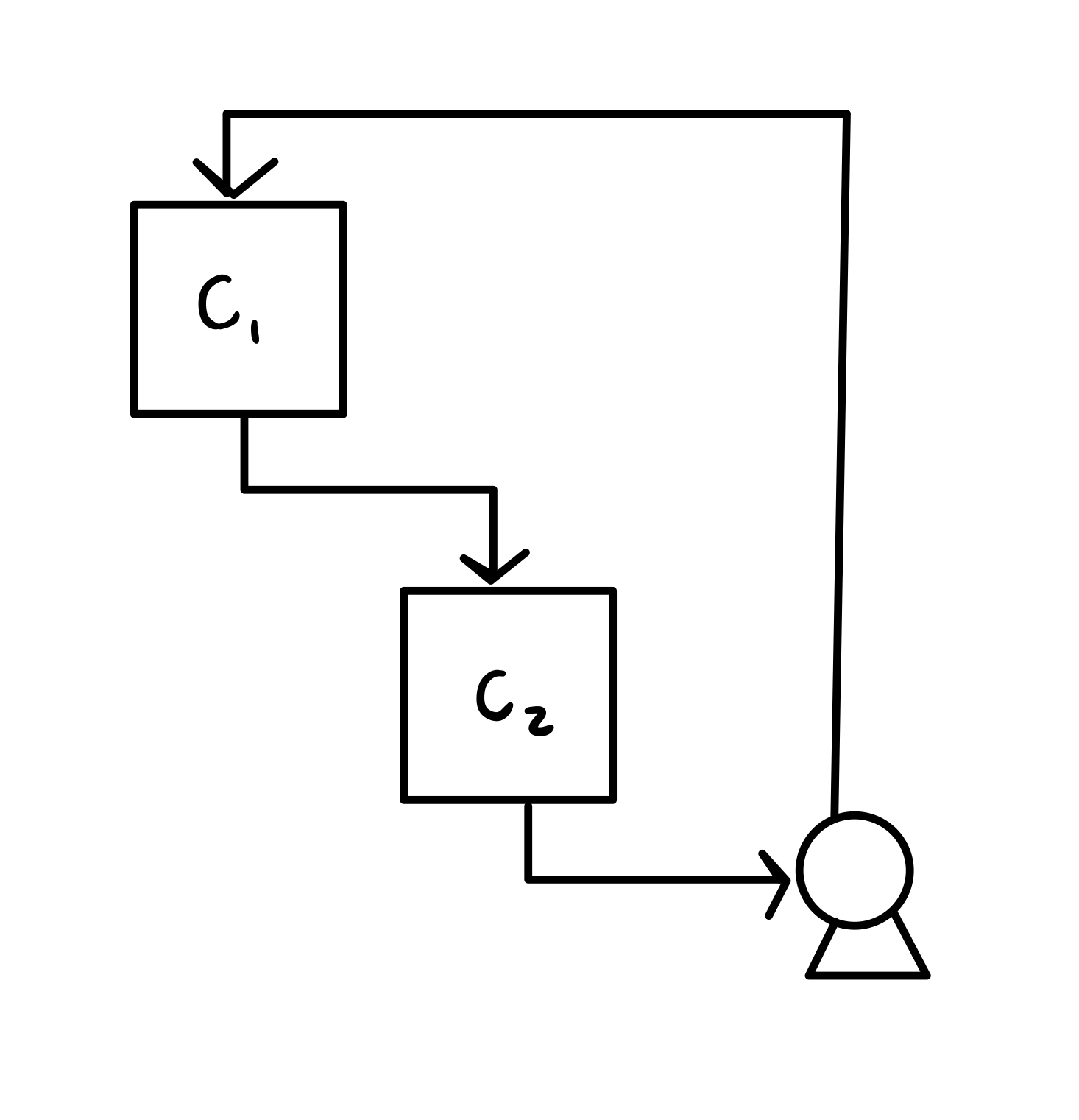
For example, consider two tanks. Tank 1 has concentration c 1 c_1 c 1 c 2 c_2 c 2
Eventually, the two concentrations should equalize, but how do they evolve to
over time? c 1 c_1 c 1 c 2 c_2 c 2 system of first-order ODEs that can be solved simultaneously.
The general, explicit form of a system of first-order ODEs is:
y 1 ′ = f 1 ( t , y 1 , ⋯ , y n ) ⋮ y n ′ = f n ( t , y 1 , ⋯ , y n ) \begin{align}
y_1' &= f_1(t, y_1, \cdots, y_n)\\
\vdots \\
y_n' &= f_n(t, y_1, \cdots, y_n)
\end{align} y 1 ′ ⋮ y n ′ = f 1 ( t , y 1 , ⋯ , y n ) = f n ( t , y 1 , ⋯ , y n ) where t is the independent variable, ( y 1 , ⋯ , y n ) (y_1, \cdots, y_n) ( y 1 , ⋯ , y n ) n
dependent variables, and ( f 1 , ⋯ , f n ) (f_1, \cdots, f_n) ( f 1 , ⋯ , f n ) n right-hand side
functions of the n ODEs. We will notate this system more compactly using
vectors
y ′ = f ( t , y ) \vv{y}' = \vv{f}(t, \vv{y}) y ′ = f ( t , y ) where y is the column vector of dependent variables, f is the column
vector of right-hand side functions, and y ′ \vv{y}' y ′
Successive substitution ¶ Some systems of first-order ODEs have a special structure that allows you to
solve one equation at a time, then substitute into another that can now be
solved. This process can be repeated successively to solve for all dependent
variables.
Example: Reaction network ¶ We are analyzing a simple reaction sequence occuring in a batch reactor:
A → k 1 B → k 2 C {\rm A} \xrightarrow{k_1} {\rm B} \xrightarrow{k_2} {\rm C} A k 1 B k 2 C where k 1 k_1 k 1 k 2 k_2 k 2 t = 0 t = 0 t = 0 c A , 0 c_{{\rm A},0} c A , 0 k 1 = k 2 k_1 = k_2 k 1 = k 2
Unsteady mole balances give
d c A d t = − k 1 c A d c B d t = k 1 c A − k 2 c B d c C d t = k 2 c B \begin{align}
\dd{}{c_{\rm A}}{t} &= -k_1 c_{\rm A} \\
\dd{}{c_{\rm B}}{t} &= k_1 c_{\rm A} - k_2 c_{\rm B} \\
\dd{}{c_{\rm C}}{t} &= k_2 c_{\rm B}
\end{align} d t d c A d t d c B d t d c C = − k 1 c A = k 1 c A − k 2 c B = k 2 c B These ODES can be solved by first finding c A c_{\rm A} c A c B c_{\rm B} c B c C c_{\rm C} c C c A c_{\rm A} c A
∫ d c A c A = ∫ − k 1 d t ln c A = − k 1 t + K \begin{align}
\int \frac{\d{c_{\rm A}}}{c_{\rm A}} &= \int -k_1 \d{t} \\
\ln c_{\rm A} &= -k_1 t + K
\end{align} ∫ c A d c A ln c A = ∫ − k 1 d t = − k 1 t + K Applying the initial condition c A ( 0 ) = c A , 0 c_{\rm A}(0) = c_{{\rm A},0} c A ( 0 ) = c A , 0
c A = c A , 0 e − k 1 t c_{\rm A} = c_{{\rm A}, 0} e^{-k_1 t} c A = c A , 0 e − k 1 t Next, use the solution for c A c_{\rm A} c A c B c_{\rm B} c B
d c B d t = k 1 c A , 0 e − k 1 t − k 2 c B d c B d t + k 2 c B = k 1 c A , 0 e − k 1 t \begin{align}
\dd{}{c_{\rm B}}{t} &= k_1 c_{\rm A,0}e^{-k_1 t} -k_2 c_{\rm B} \\
\dd{}{c_{\rm B}}{t} &+ k_2 c_{\rm B} = k_1 c_{\rm A,0}e^{-k_1 t}
\end{align} d t d c B d t d c B = k 1 c A , 0 e − k 1 t − k 2 c B + k 2 c B = k 1 c A , 0 e − k 1 t This is a linear first-order ODE with
p = k 2 r = k 1 c A , 0 e − k 1 t p = k_2 \qquad r =k_1 c_{\rm A,0}e^{-k_1 t} p = k 2 r = k 1 c A , 0 e − k 1 t that can be solved using an integrating factor:
F = e ∫ k 2 d t = e k 2 t ∫ F r d t = ∫ e k 2 t k 1 c A , 0 e − k 1 t d t = k 1 c A , 0 ∫ e ( k 2 − k 1 ) t d t = c A , 0 k 1 k 2 − k 1 e ( k 2 − k 1 ) t \begin{align}
F &= e^{\int k_2 \d{t}} = e^{k_2 t} \\
\int F r \d{t} &= \int e^{k_2 t} k_1 c_{\rm A,0} e^{-k_1 t} \d{t} \\
&= k_1 c_{\rm A,0} \int e^{(k_2 -k_1)t} \d{t} \\
&= c_{\rm A,0} \frac{k_1}{k_2 -k_1} e^{(k_2 -k_1)t}
\end{align} F ∫ F r d t = e ∫ k 2 d t = e k 2 t = ∫ e k 2 t k 1 c A , 0 e − k 1 t d t = k 1 c A , 0 ∫ e ( k 2 − k 1 ) t d t = c A , 0 k 2 − k 1 k 1 e ( k 2 − k 1 ) t Hence,
c B = 1 F ( ∫ F r d t + K ) = c A , 0 k 1 k 2 − k 1 e − k 1 t + K e − k 2 t \begin{align}
c_{\rm B} &= \frac{1}{F}\left(\int Fr\d{t} + K \right) \\
&= c_{\rm A,0} \frac{k_1}{k_2 - k_1} e^{-k_1 t} + K e^{-k_2 t}
\end{align} c B = F 1 ( ∫ F r d t + K ) = c A , 0 k 2 − k 1 k 1 e − k 1 t + K e − k 2 t Applying the initial condition
c B ( 0 ) = c A , 0 k 1 k 2 − k 1 + K = 0 K = − c A , 0 k 1 k 2 − k 1 \begin{align}
c_{\rm B}(0) &= c_{\rm A,0} \frac{k_1}{k_2 - k_1} + K = 0 \\
K &= -c_{\rm A,0} \frac{k_1}{k_2 - k_1}
\end{align} c B ( 0 ) K = c A , 0 k 2 − k 1 k 1 + K = 0 = − c A , 0 k 2 − k 1 k 1 Hence,
c B = c A , 0 k 1 k 2 − k 1 ( e − k 1 t − e − k 2 t ) c_{\rm B} = c_{\rm A,0} \frac{k_1}{k_2 -k_1} \left(e^{-k_1 t} - e^{-k_2 t} \right) c B = c A , 0 k 2 − k 1 k 1 ( e − k 1 t − e − k 2 t ) If k 1 = k 2 k_1 = k_2 k 1 = k 2 k 1 = k k_1 = k k 1 = k k 2 → k k_2 \to k k 2 → k
lim k 2 → k c B = c A , 0 k lim k 2 → k e − k t − e − k 2 t k 2 − k 1 = c A , 0 k lim k 2 → k t e − k 2 t 1 = c A , 0 k t e − k t \begin{align}
\lim_{k_2 \to k} c_{\rm B} &=
c_{{\rm A},0} k \lim_{k_2 \to k} \frac{e^{-k t} - e^{-k_2 t}}{k_2 -k_1} \\
&= c_{{\rm A},0} k \lim_{k_2 \to k} \frac{t e^{-k_2 t}}{1} \\
&= c_{{\rm A},0} k t e^{-k t}
\end{align} k 2 → k lim c B = c A , 0 k k 2 → k lim k 2 − k 1 e − k t − e − k 2 t = c A , 0 k k 2 → k lim 1 t e − k 2 t = c A , 0 k t e − k t where in the second line, we made use of L’Hopital’s rule to evaluate the limit.
Skill builder problems ¶ Solve the IVP
y 1 ′ = 1 − 2 y 1 , y 1 ( 0 ) = 0 y 2 ′ = 2 y 1 − y 1 y 2 , y 2 ( 0 ) = 0 \begin{align}
y_1' &= 1-2y_1, & y_1(0) &= 0\\
y_2' &= 2y_1 - y_1y_2, & y_2(0) &= 0
\end{align} y 1 ′ y 2 ′ = 1 − 2 y 1 , = 2 y 1 − y 1 y 2 , y 1 ( 0 ) y 2 ( 0 ) = 0 = 0 We begin by solving for y 1 y_1 y 1 x . The ODE is separable and
therefore can be solved using separation of variables.
∫ d y 1 1 − 2 y 1 = ∫ d x − 1 2 ln ( 1 − 2 y 1 ) = x + c 0 ln ( 1 − 2 y 1 ) = − 2 x + c 1 1 − 2 y 1 = c 2 e − 2 x y 1 = 1 2 ( 1 − c 2 e − 2 x ) \begin{align}
\int \frac{dy_1}{1-2y_1} &= \int dx \\
-\frac{1}{2} \ln{\left(1-2y_1\right)} &= x + c_0 \\
\ln{\left(1-2y_1\right)} &= -2x + c_1 \\
1 - 2y_1 &= c_2 e^{-2x} \\
y_1 &= \frac{1}{2} \left(1- c_2 e^{-2x}\right) \\
\end{align} ∫ 1 − 2 y 1 d y 1 − 2 1 ln ( 1 − 2 y 1 ) ln ( 1 − 2 y 1 ) 1 − 2 y 1 y 1 = ∫ d x = x + c 0 = − 2 x + c 1 = c 2 e − 2 x = 2 1 ( 1 − c 2 e − 2 x ) Now, use the initial condition y 1 ( 0 ) = 0 y_1(0)= 0 y 1 ( 0 ) = 0 c 2 c_2 c 2
y 1 ( 0 ) = 1 2 ( 1 − c 2 ) = 0 y_1(0) = \frac{1}{2}\left(1-c_2\right) = 0 y 1 ( 0 ) = 2 1 ( 1 − c 2 ) = 0 so c 2 = 1 c_2 = 1 c 2 = 1
y 1 = 1 2 ( 1 − e − 2 x ) y_1 = \frac{1}{2} \left(1-e^{-2x}\right) y 1 = 2 1 ( 1 − e − 2 x ) Now, we can solve for y 2 y_2 y 2 y 1 y_1 y 1 y 2 y_2 y 2
y 2 ′ = y 1 ( 2 − y 2 ) ∫ d y 2 2 − y 2 = ∫ 1 2 ( 1 − e − 2 x ) d x − ln ( 2 − y 2 ) = 1 2 ( x + 1 2 e − 2 x ) + c 0 2 − y 2 = c 1 exp [ − 1 2 ( x + 1 2 e − 2 x ) ] y 2 = 2 − c 1 exp [ − 1 2 ( x + 1 2 e − 2 x ) ] \begin{align}
y_2' &= y_1\left(2-y_2\right) \\
\int \frac{dy_2}{2-y_2} &= \int \frac{1}{2}\left(1-e^{-2x}\right) \d{x} \\
-\ln{\left(2-y_2\right)} &= \frac{1}{2}\left(x + \frac{1}{2}e^{-2x}\right) + c_0\\
2 - y_2
&= c_1 \exp\left[-\frac{1}{2}\left(x+ \frac{1}{2}e^{-2x}\right)\right] \\
y_2
&= 2 - c_1 \exp\left[-\frac{1}{2}\left(x+\frac{1}{2}e^{-2x}\right)\right] \\
\end{align} y 2 ′ ∫ 2 − y 2 d y 2 − ln ( 2 − y 2 ) 2 − y 2 y 2 = y 1 ( 2 − y 2 ) = ∫ 2 1 ( 1 − e − 2 x ) d x = 2 1 ( x + 2 1 e − 2 x ) + c 0 = c 1 exp [ − 2 1 ( x + 2 1 e − 2 x ) ] = 2 − c 1 exp [ − 2 1 ( x + 2 1 e − 2 x ) ] Again, use the initial condition y 2 ( 0 ) = 0 y_2(0)= 0 y 2 ( 0 ) = 0 c 1 c_1 c 1
y 2 ( 0 ) = 2 − c 1 e − 1 / 4 = 0 c 1 = 2 e 1 / 4 \begin{align}
y_2(0) &= 2 - c_1 e^{-1/4} = 0 \\
c_1 &= 2e^{1/4}
\end{align} y 2 ( 0 ) c 1 = 2 − c 1 e − 1/4 = 0 = 2 e 1/4 Therefore,
y 2 = 2 [ 1 − exp ( 1 4 − x 2 − 1 4 e − 2 x ) ] y_2 = 2\left[1-\exp\left(\frac{1}{4}-\frac{x}{2}-\frac{1}{4}e^{-2x}\right)\right] y 2 = 2 [ 1 − exp ( 4 1 − 2 x − 4 1 e − 2 x ) ]