7.1 Substitution
Some second-order ODEs can be solved by making a substitution
u = d y d x u = \dd{}{y}{x} u = d x d y Then, you effectively “integrate twice”: once to solve for u , then once more
to get y from u .
Example: Kinematics ¶ Newton’s second law is F = m a F = ma F = ma F is the applied force, m is the
mass, and a is the acceleration of a body. We also know that acceleration
is the derivative of the velocity v , which is itself the first derivative
of position x . Hence, Newton’s second-law is a second-order ODE:
m d 2 x d t 2 = F m \dd{2}{x}{t} = F m d t 2 d 2 x = F Solve for the position of a body x as a function of time t experience a
constant gravitational force F = − m g F = -mg F = − m g g is the acceleration due to
gravity.
Substitute the gravitational force and simplify
m d 2 x d t 2 = − m g d 2 x d t 2 = − g \begin{align}
m \dd{2}{x}{t} &= -mg \\
\dd{2}{x}{t} &= -g
\end{align} m d t 2 d 2 x d t 2 d 2 x = − m g = − g Make the substitution v = d x / d t v = \d{x}/\d{t} v = d x / d t
d v d t = − g ∫ d v = ∫ − g d t v = − g t + c 1 \begin{align}
\dd{}{v}{t} &= -g \\
\int \d{v} &= \int -g \d{t} \\
v &= -g t + c_1
\end{align} d t d v ∫ d v v = − g = ∫ − g d t = − g t + c 1 Replace v and integrate again:
d x d t = − g t + c 1 ∫ d x = ∫ ( − g t + c 1 ) d t x = − 1 2 g t 2 + c 1 t + c 2 \begin{align}
\dd{}{x}{t} &= -g t + c_1 \\
\int \d{x} &= \int\left(-g t + c_1 \right)\d{t} \\
x &= -\frac{1}{2} g t^2 + c_1 t + c_2
\end{align} d t d x ∫ d x x = − g t + c 1 = ∫ ( − g t + c 1 ) d t = − 2 1 g t 2 + c 1 t + c 2 If the initial position is x ( 0 ) = x 0 x(0) = x_0 x ( 0 ) = x 0 v ( 0 ) = x ′ ( 0 ) = v 0 v(0)=x'(0)=v_0 v ( 0 ) = x ′ ( 0 ) = v 0
x ( 0 ) = c 2 = x 0 v ( 0 ) = c 1 = v 0 \begin{align}
x(0) &= c_2 = x_0 \\
v(0) &= c_1 = v_0
\end{align} x ( 0 ) v ( 0 ) = c 2 = x 0 = c 1 = v 0 so
x ( t ) = − 1 2 g t 2 + v 0 t + x 0 x(t) = -\frac{1}{2} g t^2 + v_0 t + x_0 x ( t ) = − 2 1 g t 2 + v 0 t + x 0 This is the classic equation of ballistic motion!
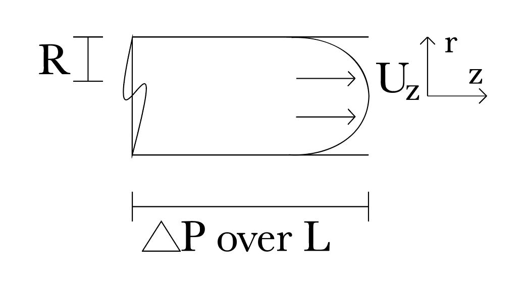
Example: Incompressible flow in a cylinder ¶ Steady, laminar pressure-driven flow in a cylindrical pipe:
is governed by the simplified Navier-Stokes equation:
μ 1 r d d r ( r d u z d r ) = − Δ P L \mu \frac{1}{r} \dd{}{}{r} \left( r \dd{}{u_z}{r} \right) = -\frac{\Delta P}{L} μ r 1 d r d ( r d r d u z ) = − L Δ P where u z u_z u z Δ P \Delta P Δ P L is the length of the
pipe, and μ \mu μ
The pipe walls have no-slip boundary conditions, meaning the velocity is zero
there. Derive an expression for u z ( r ) u_z(r) u z ( r )
Make the substitution v = r d u z / d r v = r \d{u_z}/\d{r} v = r d u z / d r
μ 1 r d v d r = − Δ P μ L ∫ d v = ∫ − 1 μ Δ P L r d r v = − 1 2 μ Δ P L r 2 + c 1 \begin{align}
\mu \frac{1}{r} \dd{}{v}{r} &= -\frac{\Delta P}{\mu L} \\
\int \d{v} &= \int -\frac{1}{\mu} \frac{\Delta P}{L} r \d{r} \\
v &= -\frac{1}{2\mu} \frac{\Delta P}{L} r^2 + c_1
\end{align} μ r 1 d r d v ∫ d v v = − μL Δ P = ∫ − μ 1 L Δ P r d r = − 2 μ 1 L Δ P r 2 + c 1 Then, substitute for v , separate, and integrate again:
r d u z d r = − 1 2 μ Δ P L r 2 + c 1 ∫ d u z = ∫ ( − 1 2 μ Δ P L r + c 1 r ) d r u z = − 1 4 μ Δ P L r 2 + c 1 ln r + c 2 \begin{align}
r \dd{}{u_z}{r} &= -\frac{1}{2\mu} \frac{\Delta P}{L} r^2 + c_1 \\
\int \d{u_z} &= \int \Biggl( -\frac{1}{2\mu} \frac{\Delta P}{L} r +
\frac{c_1}{r} \Biggr) \d{r} \\
u_z &= -\frac{1}{4\mu} \frac{\Delta P}{L} r^2 + c_1 \ln r + c_2
\end{align} r d r d u z ∫ d u z u z = − 2 μ 1 L Δ P r 2 + c 1 = ∫ ( − 2 μ 1 L Δ P r + r c 1 ) d r = − 4 μ 1 L Δ P r 2 + c 1 ln r + c 2 The walls have no-slip boundary conditions so u z ( R ) = 0 u_z(R) = 0 u z ( R ) = 0 u z ′ ( 0 ) = 0 u_z'(0) = 0 u z ′ ( 0 ) = 0
lim r → 0 u z ′ ( r ) = lim r → 0 c 1 r = 0 u z ( R ) = − 1 4 μ Δ P L R 2 + c 1 ln R + c 2 = 0 \begin{align}
\lim_{r \to 0} u_z'(r) &= \lim_{r \to 0} \frac{c_1}{r} = 0 \\
u_z(R) &= -\frac{1}{4\mu} \frac{\Delta P}{L} R^2 + c_1 \ln R + c_2 = 0
\end{align} r → 0 lim u z ′ ( r ) u z ( R ) = r → 0 lim r c 1 = 0 = − 4 μ 1 L Δ P R 2 + c 1 ln R + c 2 = 0 The first equation requires c 1 = 0 c_1 = 0 c 1 = 0
c 2 = 1 4 μ Δ P L R 2 c_2 = \frac{1}{4\mu} \frac{\Delta P}{L} R^2 c 2 = 4 μ 1 L Δ P R 2 All together,
u z ( r ) = 1 4 μ Δ P L ( R 2 − r 2 ) u_z(r)=\frac{1}{4 \mu}\frac{\Delta P}{L}(R^2-r^2) u z ( r ) = 4 μ 1 L Δ P ( R 2 − r 2 ) This is the classic Hagen-Poiseuille flow profile.