7.7 Numerical solution methods
Initial value problems ¶ We learned previously how to solve systems of first-order ODEs:
y ′ = f ( t , y ) \vv{y}' = \vv{f}(t, \vv{y}) y ′ = f ( t , y ) using Euler’s method. However, we didn’t learn what to do with higher-order
derivatives. If a second-order ODE can be written in explicit form and as an
initial value problem:
y ′ ′ = f ( t , y , y ′ ) , y ( 0 ) = y 0 , y ′ ( 0 ) = y 0 ′ y'' = f(t, y, y'), \quad y(0) = y_0, \quad y'(0) = y_0' y ′′ = f ( t , y , y ′ ) , y ( 0 ) = y 0 , y ′ ( 0 ) = y 0 ′ it can be solved by conversion to a system of first-order ODEs!
Conversion to a system of first-order ODEs
For the explicit second-order ODE y ′ ′ = f ( t , y , y ′ ) y'' = f(t, y, y') y ′′ = f ( t , y , y ′ ) y 1 = y y_1 = y y 1 = y y 2 = y ′ y_2 = y' y 2 = y ′
y 1 ′ = y 2 , y 1 ( 0 ) = y ( 0 ) y 2 ′ = f ( t , y 1 , y 2 ) , y 2 ( 0 ) = y ′ ( 0 ) \begin{align}
y_1' &= y_2, & y_1(0) &= y(0)\\
y_2' &= f(t, y_1, y_2), & y_2(0) &= y'(0)
\end{align} y 1 ′ y 2 ′ = y 2 , = f ( t , y 1 , y 2 ) , y 1 ( 0 ) y 2 ( 0 ) = y ( 0 ) = y ′ ( 0 ) Note: this procedure actually works for even higher-order ODEs! The size of the
system is equal to the highest derivative.
Let’s verify this works using an ODE that we can solve analytically. Consider:
y ′ ′ + y ′ − 2 y = 0 y ( 0 ) = 4 , y ′ ( 0 ) = − 5 y'' + y' - 2y = 0 \quad y(0) = 4, \quad y'(0) = -5 y ′′ + y ′ − 2 y = 0 y ( 0 ) = 4 , y ′ ( 0 ) = − 5 We previously showed using the
characteristic polynomial that the
solution to this IVP is:
y = e x + 3 e − 2 x y = e^x + 3e^{-2x} y = e x + 3 e − 2 x Now, let’s resolve by converting to a system. Let y 1 = y y_1 = y y 1 = y y 2 = y ′ y_2 = y' y 2 = y ′
y ′ ′ = 2 y − y ′ y 2 ′ = 2 y 1 − y 2 \begin{align}
y'' &= 2y - y' \\
y_2' &= 2y_1 - y_2
\end{align} y ′′ y 2 ′ = 2 y − y ′ = 2 y 1 − y 2 and the system of ODEs is:
y 1 ′ = y 2 , y 1 ( 0 ) = 4 y 2 ′ = 2 y 1 + − y 2 , y 2 ( 0 ) = − 5 \begin{align}
y_1' &= y_2, & y_1(0) &= 4 \\
y_2' &= 2y_1 + -y_2, & y_2(0) &= -5
\end{align} y 1 ′ y 2 ′ = y 2 , = 2 y 1 + − y 2 , y 1 ( 0 ) y 2 ( 0 ) = 4 = − 5 This system of ODES is in the form y ′ = A y \vv{y}' = \vv{A}\vv{y} y ′ = Ay
[ 0 1 2 − 1 ] \begin{bmatrix} 0 & 1 \\ 2 & -1\end{bmatrix} [ 0 2 1 − 1 ] The eigenvalues of the matrix are
∣ A − λ I ∣ = ∣ − λ 1 2 − 1 − λ ∣ = λ ( λ + 1 ) − 2 = λ 2 + λ − 2 = ( λ − 1 ) ( λ + 2 ) = 0 \begin{align}
|\vv{A}-\lambda \vv{I}|
&=\begin{vmatrix}-\lambda & 1\\ 2& -1-\lambda \end{vmatrix} \\
&=\lambda(\lambda+1)-2 \\
&= \lambda^2 + \lambda - 2 \\
&= (\lambda-1)(\lambda+2) = 0
\end{align} ∣ A − λ I ∣ = ∣ ∣ − λ 2 1 − 1 − λ ∣ ∣ = λ ( λ + 1 ) − 2 = λ 2 + λ − 2 = ( λ − 1 ) ( λ + 2 ) = 0 giving λ 1 = 1 \lambda_1 = 1 λ 1 = 1 λ 2 = − 2 \lambda_2 = -2 λ 2 = − 2
A − λ 1 I = [ − 1 1 2 − 2 ] → x 1 = [ 1 1 ] A − λ 2 I = [ 2 1 2 1 ] → x 2 = [ 1 − 2 ] \begin{align}
\vv{A} - \lambda_1 \vv{I} &=
\begin{bmatrix} -1 & 1 \\ 2 & -2 \end{bmatrix} \to \vv{x}_1 =
\begin{bmatrix}1 \\ 1\end{bmatrix} \\
\vv{A} - \lambda_2 \vv{I} &=
\begin{bmatrix} 2 & 1 \\ 2 & 1 \end{bmatrix} \to \vv{x}_2 =
\begin{bmatrix}1 \\ -2\end{bmatrix}
\end{align} A − λ 1 I A − λ 2 I = [ − 1 2 1 − 2 ] → x 1 = [ 1 1 ] = [ 2 2 1 1 ] → x 2 = [ 1 − 2 ] Hence,
y = c 1 e x [ 1 1 ] + c 2 e − 2 x [ 1 − 2 ] \vv{y} = c_1 e^x \begin{bmatrix}1 \\ 1\end{bmatrix} +
c_2 e^{-2x} \begin{bmatrix}1 \\ -2\end{bmatrix} y = c 1 e x [ 1 1 ] + c 2 e − 2 x [ 1 − 2 ] Apply the initial conditions by solving X c = y ( 0 ) \vv{X} \vv{c} = \vv{y}(0) Xc = y ( 0 )
[ 1 1 4 1 − 2 − 5 ] R 1 − R 1 → [ 1 1 4 0 − 3 − 9 ] R 1 ÷ − 3 → [ 1 1 4 0 1 3 ] − R 2 R 2 → [ 1 0 1 0 1 3 ] \begin{align}
\begin{bmatrix}1 & 1 & 4 \\ 1 & -2 & -5 \end{bmatrix}
\begin{matrix}\vphantom{R_1} \\ -R_1\end{matrix}
&\to \begin{bmatrix}1 & 1 & 4 \\ 0 & -3 & -9 \end{bmatrix}
\begin{matrix}\vphantom{R_1} \\ \div -3\end{matrix} \\
&\to \begin{bmatrix}1 & 1 & 4 \\ 0 & 1 & 3 \end{bmatrix}
\begin{matrix} -R_2 \\ \vphantom{R_2}\end{matrix} \\
&\to \begin{bmatrix}1 & 0 & 1 \\ 0 & 1 & 3 \end{bmatrix}
\end{align} [ 1 1 1 − 2 4 − 5 ] R 1 − R 1 → [ 1 0 1 − 3 4 − 9 ] R 1 ÷ − 3 → [ 1 0 1 1 4 3 ] − R 2 R 2 → [ 1 0 0 1 1 3 ] so
y = e x [ 1 1 ] + 3 e − 2 x [ 1 − 2 ] \vv{y} = e^x \begin{bmatrix}1 \\ 1\end{bmatrix} +
3 e^{-2x} \begin{bmatrix}1 \\ -2\end{bmatrix} y = e x [ 1 1 ] + 3 e − 2 x [ 1 − 2 ] or equivalently
y = y 1 = e x + 3 e − 2 x y = y_1 = e^x + 3 e^{-2x} y = y 1 = e x + 3 e − 2 x The solution is the same as before! Note that in the process, we also obtained
y ′ = y 2 = e x − 6 e − 2 x y' = y_2 = e^x - 6 e^{-2x} y ′ = y 2 = e x − 6 e − 2 x which is consistent with direct differentiation of y y y
Example: Forced oscillator ¶ A mass m on a Hookean spring (constant k ) is experiences both a drag force
(friction coefficient γ \gamma γ F cos ω t F \cos \omega t F cos ω t x obeys the differential equation
m x ′ ′ + γ x ′ + k x = F cos ω t , x ( 0 ) = x 0 , x ′ ( 0 ) = v 0 m x'' + \gamma x' + kx = F \cos\omega t, \quad x(0) = x_0, \quad x'(0) = v_0 m x ′′ + γ x ′ + k x = F cos ω t , x ( 0 ) = x 0 , x ′ ( 0 ) = v 0 where x 0 x_0 x 0 v 0 v_0 v 0
Let y 1 = x y_1 = x y 1 = x y 2 = x ′ y_2 = x' y 2 = x ′
x ′ ′ = 1 m ( − k x − γ x ′ + F cos ω t ) y 2 ′ = 1 m ( − k y 1 − γ y 2 + F cos ω t ) \begin{align}
x'' = \frac{1}{m}\left(- kx - \gamma x' + F\cos\omega t\right) \\
y_2' = \frac{1}{m}\left(- k y_1 - \gamma y_2 + F\cos \omega t \right)
\end{align} x ′′ = m 1 ( − k x − γ x ′ + F cos ω t ) y 2 ′ = m 1 ( − k y 1 − γ y 2 + F cos ω t ) so
y 1 ′ = y 2 , y 1 ( 0 ) = x 0 y 2 ′ = 1 m ( − γ y 2 − k y 1 + F cos ω t ) , y 2 ( 0 ) = v 0 \begin{align}
y_1' &= y_2, & y_1(0) &= x_0 \\
y_2' &= \displaystyle
\frac{1}{m}\left(-\gamma y_2 - k y_1 + F\cos \omega t \right), &
y_2(0) &= v_0
\end{align} y 1 ′ y 2 ′ = y 2 , = m 1 ( − γ y 2 − k y 1 + F cos ω t ) , y 1 ( 0 ) y 2 ( 0 ) = x 0 = v 0 Boundary value problems ¶ We can solve initial value problems for second-order ODEs by converting to a
system and using methods we know. What about boundary value problems?
Let’s say we want to solve:
y ′ ′ + y = 0 , y ( 0 ) = 0 , y ( π / 6 ) = 4 y'' + y = 0, \quad y(0) = 0, \quad y(\pi/6) = 4 y ′′ + y = 0 , y ( 0 ) = 0 , y ( π /6 ) = 4 Using normal approach:
y = c 1 cos x + c 2 sin x y ( 0 ) = c 1 = 0 y ( π / 6 ) = c 2 1 2 = 4 → c 2 = 8 \begin{align}
y &= c_1 \cos x + c_2 \sin x \\
y(0) &= c_1 = 0\\
y(\pi/6) &= c_2 \frac{1}{2} = 4 \to c_2 = 8\\
\end{align} y y ( 0 ) y ( π /6 ) = c 1 cos x + c 2 sin x = c 1 = 0 = c 2 2 1 = 4 → c 2 = 8 so,
y = 8 sin x y = 8 \sin x y = 8 sin x What if we needed to do this numerically? Try converting to system using
y 1 = y y_1 = y y 1 = y y 2 = y ′ y_2 = y' y 2 = y ′
y ′ ′ + y = 0 → y 2 ′ = − y 1 y'' + y = 0 \to y_2' = -y_1 y ′′ + y = 0 → y 2 ′ = − y 1 and
y 1 ′ = y 2 , y 1 ( 0 ) = 0 y 2 ′ = − y 1 , y 2 ( 0 ) = a \begin{align}
y_1' &= y_2, & y_1(0) &= 0 \\
y_2' &= -y_1, & y_2(0) &= a
\end{align} y 1 ′ y 2 ′ = y 2 , = − y 1 , y 1 ( 0 ) y 2 ( 0 ) = 0 = a where a is an unknown value that we need to figure out so that y ( π / 6 ) = 4 y(\pi/6) = 4 y ( π /6 ) = 4
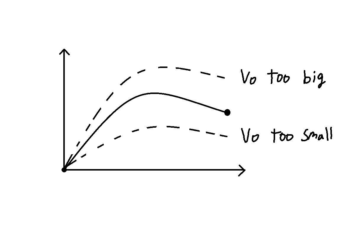
We will use the shooting method to determine a . The idea is to treat the
boundary condition at the other value of x as a function of a , then vary a
using a root-finding approach.
This boundary-condition function is the numerical integration of the system of
ODEs! Bisection search is well-suited for solving for a because it is stable
and doesn’t require a derivative.
Example: Reaction-diffusion with second-order reaction ¶ We are solving a reaction-diffusion problem with a second-order reaction:
D d 2 c d x 2 − k c 2 = 0 , c ( 0 ) = c 0 , − D c ′ ( L ) = 0 D \dd{2}{c}{x} - k c^2 = 0, \quad c(0) = c_0, \quad -D c'(L) = 0 D d x 2 d 2 c − k c 2 = 0 , c ( 0 ) = c 0 , − D c ′ ( L ) = 0 Formulate in a form suitable for numerical solution using the shooting method.
First, rewrite as a system of first-order ODEs using y 1 = c y_1 = c y 1 = c c 2 = c ′ c_2 = c' c 2 = c ′
c ′ ′ − k D c 2 → y 2 ′ = k D y 1 2 c'' - \frac{k}{D}c^2 \to y_2' = \frac{k}{D} y_1^2 c ′′ − D k c 2 → y 2 ′ = D k y 1 2 so
y 1 ′ = y 2 , y 1 ( 0 ) = c 0 y 2 ′ = k D y 1 , y 2 ( 0 ) = a \begin{align}
y_1' &= y_2, & y_1(0) &= c_0 \\
y_2' &= \frac{k}{D} y_1, & y_2(0) &= a
\end{align} y 1 ′ y 2 ′ = y 2 , = D k y 1 , y 1 ( 0 ) y 2 ( 0 ) = c 0 = a where a is the unknown value of y 2 ( 0 ) y_2(0) y 2 ( 0 ) a until
− D c ′ ( L ) = 0 → y 2 ( L ) = 0 -D c'(L) = 0 \to y_2(L) = 0 − D c ′ ( L ) = 0 → y 2 ( L ) = 0