7.4 Homogeneous linear second-order ODEs with constant coefficients
Equations of the form:
y ′ ′ + a y ′ + b y = 0 y'' + ay' + by = 0 y ′′ + a y ′ + b y = 0 come up often in chemical engineering, particularly in steady-state heat and
mass diffusion, so it is important to know how to solve them!
Guess a solution y = e λ x y=e^{\lambda x} y = e λ x
λ 2 e λ x + a ( λ e λ x ) + b e λ x = 0 λ 2 + a λ + b = 0 \begin{align}
\lambda^2 e^{\lambda x} + a (\lambda e^{\lambda x}) + b e^{\lambda x} &= 0\\
\lambda^2 + a \lambda + b &= 0
\end{align} λ 2 e λ x + a ( λ e λ x ) + b e λ x λ 2 + aλ + b = 0 = 0 This characteristic polynomial has two roots λ 1 \lambda_1 λ 1 λ 2 \lambda_2 λ 2 y is obtained by superposition of both.
Homogeneous linear second-order ODEs with constant coefficients
For ODEs of the form
y ′ ′ + a y ′ + b y = 0 y'' + ay' + by = 0 y ′′ + a y ′ + b y = 0 The roots of the characteristic polynomial
λ 2 + a λ + b = 0 \lambda^2 + a \lambda + b = 0 λ 2 + aλ + b = 0 give the solution type:
λ 1 \lambda_1 λ 1 λ 2 \lambda_2 λ 2
y = c 1 e λ 1 x + c 2 e λ 2 x y = c_1 e^{\lambda_1 x} + c_2 e^{\lambda_2 x} y = c 1 e λ 1 x + c 2 e λ 2 x λ 1 , 2 = α ± i ω \lambda_{1,2} = \alpha \pm i \omega λ 1 , 2 = α ± iω
y = e α x [ c 1 cos ( ω x ) + c 2 sin ( ω x ) ] y = e^{\alpha x} \left[c_1 \cos(\omega x) + c_2 \sin(\omega x)\right] y = e αx [ c 1 cos ( ω x ) + c 2 sin ( ω x ) ] λ 1 = λ 2 = λ \lambda_1 = \lambda_2 = \lambda λ 1 = λ 2 = λ
y = ( c 1 + c 2 x ) e λ x y=(c_1 + c_2 x) e^{\lambda x} y = ( c 1 + c 2 x ) e λ x We will consider an example of each case next.
Real distinct roots ¶ To solve
y ′ ′ + y ′ − 2 y = 0 , y ( 0 ) = 4 , y ′ ( 0 ) = − 5 y'' + y' - 2y = 0, \quad y(0)=4, \quad y'(0)=-5 y ′′ + y ′ − 2 y = 0 , y ( 0 ) = 4 , y ′ ( 0 ) = − 5 First write and solve the characteristic polynomial,
λ 2 + λ − 2 = 0 ( λ + 2 ) ( λ + 1 ) = 0 \begin{align}
\lambda^2 + \lambda -2 &= 0 \\
(\lambda + 2)(\lambda + 1) &= 0
\end{align} λ 2 + λ − 2 ( λ + 2 ) ( λ + 1 ) = 0 = 0 so λ 1 = − 2 \lambda_1 = -2 λ 1 = − 2 λ 2 = 1 \lambda_2 =1 λ 2 = 1
y = c 1 e − 2 x + c 2 e x y ′ = − 2 c 1 e − 2 x + c 2 e x \begin{align}
y &= c_1 e^{-2x} + c_2 e^{x} \\
y'&= -2c_1 e^{-2x} + c_2 e^{x} \qquad
\end{align} y y ′ = c 1 e − 2 x + c 2 e x = − 2 c 1 e − 2 x + c 2 e x So applying the initial conditions:
y ( 0 ) = c 1 + c 2 = 4 y ′ ( 0 ) = − 2 c 1 + c 2 = − 5 \begin{align}
y(0) &= c_1 + c_2 = 4 \\
y'(0) &= -2c_1 + c_2 = -5
\end{align} y ( 0 ) y ′ ( 0 ) = c 1 + c 2 = 4 = − 2 c 1 + c 2 = − 5 These coefficients can be solved by Gauss-Jordan elimination:
[ 1 1 4 − 2 1 − 5 ] R 1 + 2 R 1 → [ 1 1 4 0 3 3 ] R 1 ÷ 3 → [ 1 1 4 0 1 1 ] − R 2 R 1 → [ 1 0 3 0 1 1 ] \begin{align}
\begin{bmatrix}
1 & 1 & 4 \\
-2 & 1 & -5
\end{bmatrix}
\begin{matrix}\vphantom{R_1} \\ +2 R_1 \end{matrix}
&\to
\begin{bmatrix}
1 & 1 & 4 \\
0 & 3 & 3
\end{bmatrix}
\begin{matrix}\vphantom{R_1} \\ \div 3 \end{matrix} \\
&\to
\begin{bmatrix}
1 & 1 & 4 \\
0 & 1 & 1
\end{bmatrix}
\begin{matrix} -R_2 \\ \vphantom{R_1} \end{matrix} \\
&\to
\begin{bmatrix}
1 & 0 & 3 \\
0 & 1 & 1
\end{bmatrix}
\end{align} [ 1 − 2 1 1 4 − 5 ] R 1 + 2 R 1 → [ 1 0 1 3 4 3 ] R 1 ÷ 3 → [ 1 0 1 1 4 1 ] − R 2 R 1 → [ 1 0 0 1 3 1 ] so c 1 = 3 c_1 = 3 c 1 = 3 c 2 = 1 c_2 = 1 c 2 = 1
y = 3 e − 2 x + e x y = 3 e^{-2x} + e^x y = 3 e − 2 x + e x Complex roots ¶ To solve:
y ′ ′ + 0.4 y ′ + 9.04 y = 0 , y ( 0 ) = 0 , y ′ ( 0 ) = 3 y'' + 0.4y' + 9.04y = 0, \quad y(0)=0, \quad y'(0)=3 y ′′ + 0.4 y ′ + 9.04 y = 0 , y ( 0 ) = 0 , y ′ ( 0 ) = 3 Write and solve the characteristic polynomial,
λ 2 + 0.4 λ + 9.04 = 0 λ 1 , 2 = − 0.4 ± 0. 4 2 − 4 ⋅ 9.04 2 = − 0.2 ± 3 i \begin{align}
\lambda^{2} &+ 0.4\lambda + 9.04 = 0 \\
\lambda_{1,2} &= \frac{-0.4\pm\sqrt{0.4^2- 4 \cdot 9.04}}{2} = -0.2\pm 3i
\end{align} λ 2 λ 1 , 2 + 0.4 λ + 9.04 = 0 = 2 − 0.4 ± 0. 4 2 − 4 ⋅ 9.04 = − 0.2 ± 3 i Once values of λ \lambda λ c 1 c_1 c 1
y = e − 0.2 x ( c 1 cos 3 x + c 2 sin 3 x ) y ( 0 ) = c 1 = 0 \begin{align}
y &= e^{-0.2x}(c_1\cos3x + c_2\sin3x) \\
y(0) &= c_1 = 0
\end{align} y y ( 0 ) = e − 0.2 x ( c 1 cos 3 x + c 2 sin 3 x ) = c 1 = 0 Hence the first term can be dropped from the solution. In order to solve for
c 2 c_2 c 2
y ′ = e − 0.2 x ( 3 c 2 cos 3 x ) − 0.2 e − 0.2 x c 2 sin 3 x y ′ ( 0 ) = 3 c 2 = 3 \begin{align}
y' &= e^{-0.2x}(3c_2\cos3x) - 0.2e^{-0.2x}c_2\sin 3x \\
y'(0) &= 3c_2 = 3
\end{align} y ′ y ′ ( 0 ) = e − 0.2 x ( 3 c 2 cos 3 x ) − 0.2 e − 0.2 x c 2 sin 3 x = 3 c 2 = 3 Since c 2 = 1 c_2=1 c 2 = 1
y = e − 0.2 x sin 3 x y = e^{-0.2x}\sin 3x y = e − 0.2 x sin 3 x Real repeated roots ¶ To solve:
y ′ ′ + y ′ + 1 4 y = 0 , y ( 0 ) = 3 , y ′ ( 0 ) = − 7 2 \begin{align}
y'' + y' + \frac{1}{4}y=0, \quad y(0)=3, \quad y'(0)= -\frac{7}{2}
\end{align} y ′′ + y ′ + 4 1 y = 0 , y ( 0 ) = 3 , y ′ ( 0 ) = − 2 7 Write and solve the characteristic polynomial,
λ 2 + λ + 1 4 = 0 ( λ + 1 2 ) 2 = 0 \begin{align}
\lambda^2 + \lambda + \frac{1}{4} = 0 \\
\left(\lambda + \frac{1}{2}\right)^2 = 0
\end{align} λ 2 + λ + 4 1 = 0 ( λ + 2 1 ) 2 = 0 So λ = − 1 / 2 \lambda = -1/2 λ = − 1/2
y = ( c 1 + c 2 x ) e − x / 2 y ′ = ( c 1 + c 2 x ) ( − 1 2 e − x / 2 ) + c 2 e − x / 2 \begin{align}
y &=(c_1 + c_2x)e^{-x/2} \\
y' &=(c_1 + c_2x)(-\frac{1}{2}e^{-x/2}) + c_2 e^{-x/2}
\end{align} y y ′ = ( c 1 + c 2 x ) e − x /2 = ( c 1 + c 2 x ) ( − 2 1 e − x /2 ) + c 2 e − x /2 Use the given conditions to solve for c 1 c_1 c 1 c 2 c_2 c 2
y ( 0 ) = c 1 = 3 y ′ ( 0 ) = − c 1 2 + c 2 = − 7 2 → c 2 = − 2 \begin{align}
y(0) &= c_1 = 3 \\
y'(0) &= -\frac{c_1}{2} + c_2 = -\frac{7}{2} \to c_2 = -2
\end{align} y ( 0 ) y ′ ( 0 ) = c 1 = 3 = − 2 c 1 + c 2 = − 2 7 → c 2 = − 2 The final solution is:
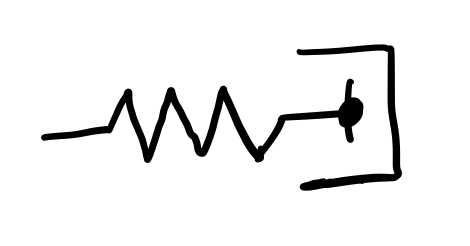
y = ( 3 − 2 x ) e − x / 2 y = (3-2x)e^{-x/2} y = ( 3 − 2 x ) e − x /2 Example: Spring and dashpot ¶ We are analyzing how the drag force affects the spring oscilations. This is a
mechanics example, but models like this are also used for the rheology of
viscoelastic materials.
A mass m is attached to a Hookean spring with spring constant k and
experiences a drag force as it moves with drag coefficient γ \gamma γ
If x is the displacement of the spring, the governing equation for x is
given by Newton’s equations:
m x ′ ′ + γ x ′ + k x = 0 m x'' + \gamma x' + k x = 0 m x ′′ + γ x ′ + k x = 0 The first term represents the acceleration of the mass, the second term is the
drag force, and the third term is the spring force.
For what values of γ \gamma γ
To answer this, first solve the roots of the characteristic polynomial for this
second-order ODE:
m λ 2 + γ λ + k = 0 λ 1 , 2 = − γ ± γ 2 − 4 m k 2 m \begin{align}
&m \lambda^2 + \gamma \lambda + k = 0 \\
\lambda_{1,2} &= \frac{ -\gamma \pm \sqrt{\gamma^2 - 4mk}}{2m}
\end{align} λ 1 , 2 m λ 2 + γλ + k = 0 = 2 m − γ ± γ 2 − 4 mk You will only get oscillations if λ 1 , 2 \lambda_{1,2} λ 1 , 2 γ 2 < 4 m k \gamma^2 < 4mk γ 2 < 4 mk
λ 1 , 2 = − γ 2 m ± i 2 m 4 m k − γ 2 \lambda_{1,2} = -\frac{\gamma}{2m} \pm \frac{i}{2m}\sqrt{4mk - \gamma^2} λ 1 , 2 = − 2 m γ ± 2 m i 4 mk − γ 2 so the general solution for x is:
x ( t ) = exp ( − γ 2 m t ) [ c 1 cos ( ω t ) + c 2 sin ( ω t ) ] x(t) = \exp\left(-\frac{\gamma}{2m} t \right)
\left [ c_1 \cos(\omega t)+ c_2 \sin(\omega t) \right] x ( t ) = exp ( − 2 m γ t ) [ c 1 cos ( ω t ) + c 2 sin ( ω t ) ] where ω = 4 m k − γ 2 \omega = \sqrt{4mk - \gamma^2} ω = 4 mk − γ 2 γ \gamma γ
γ \gamma γ 2 m / γ 2m/\gamma 2 m / γ γ \gamma γ
γ \gamma γ ω \omega ω
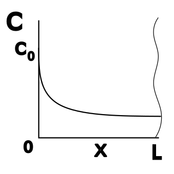
Example: Steady-state reaction-diffusion ¶ A first-order reaction is occuring in a liquid film of thickness L . The
reactant concentration at x = 0 x = 0 x = 0 c 0 c_0 c 0 x = L x=L x = L
At steady-state, the reactant concentration c can be modeled by:
D d 2 c d x 2 − k c = 0 , c ( L ) = c 0 , − D c ′ ( 0 ) = 0 \begin{align}
D \dd{2}{c}{x} -k c = 0, \quad c(L) = c_0, \quad -D c'(0) = 0
\end{align} D d x 2 d 2 c − k c = 0 , c ( L ) = c 0 , − D c ′ ( 0 ) = 0 where D is the reactant’s diffusion coefficient and k is the reaction rate
constant. Determine c ( x ) c(x) c ( x )
First, rewrite in standard form:
c ′ ′ − k D c = 0 c'' - \frac{k}{D} c = 0 c ′′ − D k c = 0 The characteristic polynomial is
λ 2 − k D = 0 λ = ± k D \begin{align}
\lambda^2 - \frac{k}{D} &= 0
\lambda &= \pm \sqrt{\frac{k}{D}}
\end{align} λ 2 − D k = 0 λ = ± D k The general solution and its first derivative are:
c = a 1 e x k / D + a 2 e − x k / D c ′ = a 1 k D e x k / D − a 2 k D e − x k / D \begin{align}
c &= a_1 e^{x \sqrt{k/D}} + a_2 e^{-x\sqrt{k/D}} \\
c' &= a_1 \sqrt{\frac{k}{D}} e^{x \sqrt{k/D}} -
a_2 \sqrt{\frac{k}{D}} e^{-x\sqrt{k/D}}
\end{align} c c ′ = a 1 e x k / D + a 2 e − x k / D = a 1 D k e x k / D − a 2 D k e − x k / D Evaluating the boundary conditions:
c ( 0 ) = a 1 + a 2 = 0 c ′ ( L ) = a 1 k D e L k / D − a 2 k D e − L k / D = 0 \begin{align}
c(0) &= a_1 + a_2 = 0 \\
c'(L) &= a_1 \sqrt{\frac{k}{D}} e^{L \sqrt{k/D}} -
a_2 \sqrt{\frac{k}{D}} e^{-L \sqrt{k/D}} = 0
\end{align} c ( 0 ) c ′ ( L ) = a 1 + a 2 = 0 = a 1 D k e L k / D − a 2 D k e − L k / D = 0 This is a linear system of equations. Solving for a 1 a_1 a 1 a 2 a_2 a 2
a 1 = c 0 1 + e 2 L k / D a 2 = c 0 1 + e − 2 L k / D a_1 = \frac{c_0}{1+e^{2L\sqrt{k/D}}} \qquad a_2 = \frac{c_0}{1+e^{-2L\sqrt{k/D}}} a 1 = 1 + e 2 L k / D c 0 a 2 = 1 + e − 2 L k / D c 0 Thus,
c = c 0 ( e x k / D 1 + e 2 L k / D + e x k / D 1 + e − 2 L k / D ) \begin{align}
c = c_0\Biggl(\frac{e^{x\sqrt{k/D}}}{1+e^{2L\sqrt{k/D}}}
+\frac{e^{x\sqrt{k/D}}}{1+e^{-2L\sqrt{k/D}}}\Biggr)
\end{align} c = c 0 ( 1 + e 2 L k / D e x k / D + 1 + e − 2 L k / D e x k / D ) Skill builder problems ¶ Solve the following:
Write and solve the characteristic polynomial:
λ 2 − 2 λ − 3 = 0 ( λ − 3 ) ( λ + 1 ) = 0 \begin{align}
\lambda^2 - 2\lambda - 3 &= 0 \\
(\lambda - 3)(\lambda + 1) &= 0
\end{align} λ 2 − 2 λ − 3 ( λ − 3 ) ( λ + 1 ) = 0 = 0 so λ 1 = 3 \lambda_1 = 3 λ 1 = 3 λ 2 = − 1 \lambda_2 = -1 λ 2 = − 1
y = c 1 e 3 t + c 2 e − t y ′ = 3 c 1 e 3 t − c 2 e − t \begin{align}
y &= c_1 e^{3t} + c_2 e^{-t} \\
y' &= 3c_1 e^{3t} - c_2 e^{-t}
\end{align} y y ′ = c 1 e 3 t + c 2 e − t = 3 c 1 e 3 t − c 2 e − t Apply the initial conditions:
y ( 0 ) = c 1 + c 2 = 2 y ′ ( 0 ) = 3 c 1 − c 2 = 14 \begin{align}
y(0) &= c_1 + c_2 = 2\\
y'(0) &= 3c_1 - c_2 = 14
\end{align} y ( 0 ) y ′ ( 0 ) = c 1 + c 2 = 2 = 3 c 1 − c 2 = 14 and solve the system for c 1 c_1 c 1 c 2 c_2 c 2
[ 1 1 2 3 − 1 14 ] R 1 − 3 R 1 → [ 1 1 2 0 − 4 8 ] R 1 ÷ − 4 → [ 1 1 2 0 1 − 2 ] − R 2 R 2 → [ 1 0 4 0 1 − 2 ] \begin{align}
\begin{bmatrix} 1 & 1 & 2 \\ 3 & -1 & 14 \end{bmatrix}
\begin{matrix}\vphantom{R_1} \\ -3 R_1 \end{matrix}
&\to \begin{bmatrix} 1 & 1 & 2 \\ 0 & -4 & 8 \end{bmatrix}
\begin{matrix}\vphantom{R_1} \\ \div -4 \end{matrix} \\
&\to \begin{bmatrix} 1 & 1 & 2 \\ 0 & 1 & -2 \end{bmatrix}
\begin{matrix} -R_2 \\ \vphantom{R_2} \end{matrix} \\
&\to \begin{bmatrix} 1 & 0 & 4 \\ 0 & 1 & -2 \end{bmatrix}
\end{align} [ 1 3 1 − 1 2 14 ] R 1 − 3 R 1 → [ 1 0 1 − 4 2 8 ] R 1 ÷ − 4 → [ 1 0 1 1 2 − 2 ] − R 2 R 2 → [ 1 0 0 1 4 − 2 ] Therefore:
y = 4 e 3 t − 2 e − t y = 4e^{3t} - 2e^{-t} y = 4 e 3 t − 2 e − t Write and solve the characteristic polynomial:
λ 2 + 2 λ + 1 = 0 ( λ + 1 ) 2 = 0 \begin{align}
\lambda^2 + 2\lambda + 1 &= 0 \\
(\lambda + 1)^2 &= 0
\end{align} λ 2 + 2 λ + 1 ( λ + 1 ) 2 = 0 = 0 so λ = − 1 \lambda = -1 λ = − 1
y = ( c 1 + c 2 t ) e − t y ′ = ( c 1 + c 2 t ) ( − e − t ) + c 2 e − t \begin{align}
y &= (c_1 + c_2 t) e^{-t} \\
y' &= (c_1 + c_2 t)(-e^{-t}) + c_2 e^{-t}
\end{align} y y ′ = ( c 1 + c 2 t ) e − t = ( c 1 + c 2 t ) ( − e − t ) + c 2 e − t Apply the initial conditions:
y ( 0 ) = c 1 = 4 y ′ ( 0 ) = − c 1 + c 2 = − 6 → c 2 = − 2 \begin{align}
y(0) &= c_1 = 4\\
y'(0) &= -c_1 + c_2 = -6 \to c_2 = -2
\end{align} y ( 0 ) y ′ ( 0 ) = c 1 = 4 = − c 1 + c 2 = − 6 → c 2 = − 2 Therefore:
y = ( 4 − 2 t ) e − t \begin{align}
y = (4 - 2t)e^{-t}
\end{align} y = ( 4 − 2 t ) e − t Write and solve the characteristic polynomial:
10 λ 2 − 50 λ + 65 = 0 λ 1 , 2 = 50 ± 5 0 2 − 4 ⋅ 10 ⋅ 65 20 = 5 ± i 2 \begin{align}
10\lambda^2 - 50\lambda + 65 &= 0 \\
\lambda_{1,2} &= \frac{50 \pm \sqrt{50^2 - 4 \cdot 10 \cdot 65}}{20} \\
&= \frac{5 \pm i}{2}
\end{align} 10 λ 2 − 50 λ + 65 λ 1 , 2 = 0 = 20 50 ± 5 0 2 − 4 ⋅ 10 ⋅ 65 = 2 5 ± i Since we have complex roots, the general solution and its first derivative
are:
y = e 5 t 2 ( c 1 cos t 2 + c 2 sin t 2 ) y ′ = e 5 t 2 ( − c 1 2 sin t 2 + c 2 2 cos t 2 ) + 5 2 e 5 t 2 ( c 1 cos t 2 + c 2 sin t 2 ) \begin{align}
y &= e^{\frac{5t}{2}}
\left(c_1 \cos\frac{t}{2} + c_2 \sin\frac{t}{2} \right) \\
y' &= e^{\frac{5t}{2}} \Biggl( -\frac{c_1}{2} \sin\frac{t}{2} +
\frac{c_2}{2} \cos\frac{t}{2} \Biggr) + \frac{5}{2}e^{\frac{5t}{2}}
\Biggl( c_1 \cos\frac{t}{2} + c_2 \sin\frac{t}{2} \Biggr)
\end{align} y y ′ = e 2 5 t ( c 1 cos 2 t + c 2 sin 2 t ) = e 2 5 t ( − 2 c 1 sin 2 t + 2 c 2 cos 2 t ) + 2 5 e 2 5 t ( c 1 cos 2 t + c 2 sin 2 t ) Apply the initial conditions:
y ( 0 ) = c 1 = 3 2 y ′ ( 0 ) = c 2 2 + 5 2 c 1 = 3 2 → c 2 = − 9 2 \begin{align}
y(0) &= c_1 = \frac{3}{2} \\
y'(0) &= \frac{c_2}{2} + \frac{5}{2}c_1 = \frac{3}{2} \to c_2 = -\frac{9}{2}
\end{align} y ( 0 ) y ′ ( 0 ) = c 1 = 2 3 = 2 c 2 + 2 5 c 1 = 2 3 → c 2 = − 2 9 Therefore:
y = e 5 t 2 ( 3 2 cos t 2 − 9 2 sin t 2 ) \begin{align}
y = e^{\frac{5t}{2}}
\left( \frac{3}{2} \cos\frac{t}{2} - \frac{9}{2} \sin\frac{t}{2} \right)
\end{align} y = e 2 5 t ( 2 3 cos 2 t − 2 9 sin 2 t ) Write and solve the characteristic polynomial:
λ 2 + π λ = 0 λ ( λ + π ) = 0 \begin{align}
\lambda^2 + \pi\lambda &= 0 \\
\lambda(\lambda + \pi) &= 0
\end{align} λ 2 + πλ λ ( λ + π ) = 0 = 0 so λ 1 = 0 \lambda_1 = 0 λ 1 = 0 λ 2 = − π \lambda_2 = -\pi λ 2 = − π
y = c 1 + c 2 e − π t y ′ = − c 2 π e − π t \begin{align}
y &= c_1 + c_2 e^{-\pi t} \\
y' &= -c_2 \pi e^{-\pi t}
\end{align} y y ′ = c 1 + c 2 e − π t = − c 2 π e − π t Apply the initial conditions:
y ( 0 ) = c 1 + c 2 = 3 y ′ ( 0 ) = − c 2 π = − π \begin{align}
y(0) &= c_1 + c_2 = 3 \\
y'(0) &= -c_2 \pi = -\pi
\end{align} y ( 0 ) y ′ ( 0 ) = c 1 + c 2 = 3 = − c 2 π = − π so c 1 = 2 c_1 = 2 c 1 = 2 c 2 = 1 c_2 = 1 c 2 = 1
y = 2 + e − π t y = 2 + e^{-\pi t} y = 2 + e − π t