1.3 Limits
Motivation ¶ What is the behavior of a function as its argument approaches a certain value?
For example, what happens to a function near boundaries of its domain? Near
“holes”? Under “extreme” cases, such as when something gets very small?
Limit (informal)
Let f ( x ) f(x) f ( x ) x 0 x_0 x 0 x 0 x_0 x 0 f ( x ) f(x) f ( x ) L L L x x x x 0 x_0 x 0 f f f L L L x x x x 0 x_0 x 0
lim x → x 0 f ( x ) = L \lim_{x \to x_0} f(x) = L x → x 0 lim f ( x ) = L Some functions have limits. For example:
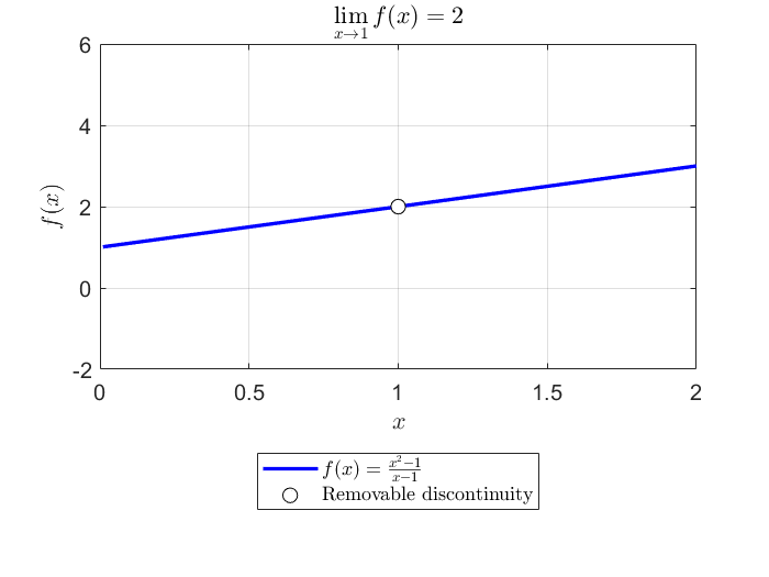
f ( x ) = x 2 − 1 x − 1 f(x) = \frac{x^2 - 1}{x - 1} f ( x ) = x − 1 x 2 − 1 is not defined when x = 1 x=1 x = 1
f ( x ) = ( x + 1 ) ( x − 1 ) x − 1 = x + 1 , x ≠ 1 f(x) = \frac{(x+1)(x-1)}{x-1} = x+1, \quad x \neq 1 f ( x ) = x − 1 ( x + 1 ) ( x − 1 ) = x + 1 , x = 1 So, we expect that f should be well-behaved and have a value that approaches
2 as x approaches 1! Let’s verify numerically:
x x x f f f 0.9 1.9 0.99 1.99 0.999 1.999 1.001 2.001 1.01 2.01 1.1 2.1
and also looking at a graph
However, some functions do not have limits. For example:
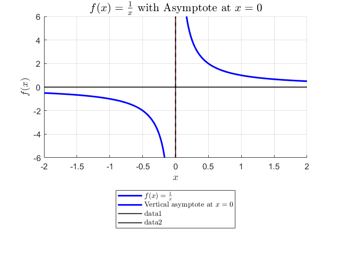
f ( x ) = 1 x f(x) = \frac{1}{x} f ( x ) = x 1 is not defined at x = 0 x = 0 x = 0 x approaches zero from the positive or negative
side, the function “blows up” to ± ∞ \pm\infty ± ∞ x
is positive or negative.
x x x f ( x ) f(x) f ( x ) 0.1 10 0.01 100 -0.01 -100 -0.1 -10
This divergence is clear on a plot:
We say that such a limit does not exist.
Limit (formal)
The limit of f f f x x x x 0 x_0 x 0 L , denoted
lim x → x 0 f ( x ) = L \lim_{x \to x_0} f(x) = L x → x 0 lim f ( x ) = L if for every ϵ > 0 \epsilon > 0 ϵ > 0 δ > 0 \delta > 0 δ > 0 x ,
if 0 < ∣ x − x 0 ∣ < δ 0 < |x-x_0| < \delta 0 < ∣ x − x 0 ∣ < δ ∣ f ( x ) − L ∣ < ϵ |f(x)-L| < \epsilon ∣ f ( x ) − L ∣ < ϵ
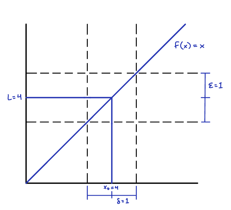
ϵ \epsilon ϵ tolerance setting how close f needs to be to L . Given
any ϵ \epsilon ϵ x values within δ \delta δ x 0 x_0 x 0 f stays within ϵ \epsilon ϵ L . For example, consider the
following:
Based on this plot, if ϵ = 1 \epsilon = 1 ϵ = 1 3 < f < 5 3 < f < 5 3 < f < 5 3 < x < 5 3 < x < 5 3 < x < 5 δ = 1 \delta = 1 δ = 1 ϵ \epsilon ϵ 4 − ϵ < f < 4 + ϵ 4 - \epsilon < f < 4 + \epsilon 4 − ϵ < f < 4 + ϵ 4 − δ < x < 4 + δ 4 - \delta < x < 4 + \delta 4 − δ < x < 4 + δ ∣ x − 4 ∣ < ϵ |x-4| < \epsilon ∣ x − 4∣ < ϵ δ = ϵ \delta = \epsilon δ = ϵ
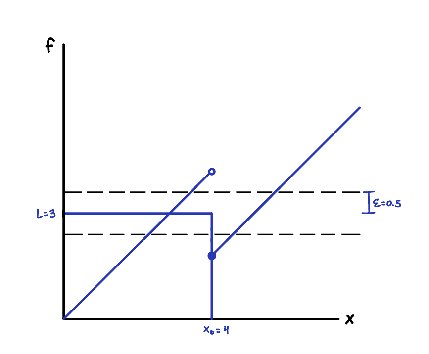
lim x → 4 f = 4 \lim_{x \to 4} f = 4 x → 4 lim f = 4 However, such a δ \delta δ ϵ \epsilon ϵ
f ( x ) = { x , x < 4 x − 2 , x ≥ 4 f(x) = \begin{cases}
x,& x < 4 \\
x-2,& x \ge 4
\end{cases} f ( x ) = { x , x − 2 , x < 4 x ≥ 4 Does the limit
lim x → 4 f ( x ) = 3 \lim_{x \to 4} f(x) = 3 x → 4 lim f ( x ) = 3 exist? If \epsilon = 0.5, there is no δ \delta δ f around
x 0 = 4 x_0 = 4 x 0 = 4
This math formalism is powerful, but clunky to apply. We will now move onto
using rules (limit laws) that have been proven using them!
Limit laws ¶ There are some simple limits and rules for combining them that are convenient
to know because they can be used to evaluate limits of more complicated
functions:
Taking limits ¶ “Nice” functions can be evaluated directly
lim x → − 1 x 3 + 4 x 2 − 3 = ( − 1 ) 3 + 4 ( − 1 ) 2 − 3 = − 1 + 4 − 3 = 0 \begin{align}
\lim_{x \to -1} x^3 + 4x^2 -3 &= (-1)^3 + 4(-1)^2 -3 \\
&= -1 + 4 -3 \\
&= 0
\end{align} x → − 1 lim x 3 + 4 x 2 − 3 = ( − 1 ) 3 + 4 ( − 1 ) 2 − 3 = − 1 + 4 − 3 = 0 This works even if they are complicated
lim x → 4 ( x 2 + 9 x + 1 ) 1 / 2 = ( 4 2 + 9 4 + 1 ) 1 / 2 = ( 25 5 ) 1 / 2 = 5 \begin{align}
\lim_{x \to 4} \left(\frac{x^2 + 9}{x + 1} \right)^{1/2}
&= \left(\frac{4^2 + 9}{4 + 1} \right)^{1/2} \\
&= \left(\frac{25}{5}\right)^{1/2} \\
&= \sqrt{5}
\end{align} x → 4 lim ( x + 1 x 2 + 9 ) 1/2 = ( 4 + 1 4 2 + 9 ) 1/2 = ( 5 25 ) 1/2 = 5 Limits are most useful when functions have “holes” (function is not defined at
x 0 x_0 x 0
lim x → 1 x 2 + x − 2 x 2 − x = lim x → 1 ( x + 2 ) ( x + 1 ) x ( x + 1 ) = lim x → 1 x + 2 x = 3 \begin{align}
\lim_{x \to 1} \frac{x^2 + x -2}{x^2 - x}
&= \lim_{x \to 1} \frac{(x+2)(x+1)}{x(x+1)} \\
&= \lim_{x \to 1} \frac{x+2}{x} \\
&= 3
\end{align} x → 1 lim x 2 − x x 2 + x − 2 = x → 1 lim x ( x + 1 ) ( x + 2 ) ( x + 1 ) = x → 1 lim x x + 2 = 3 Note that this function had a “hole” at x = 1 x = 1 x = 1
lim x → 4 4 x − x 2 2 − x = lim x → 4 x ( 4 − x ) 2 − x = lim x → 4 x ( 2 + x ) ( 2 − x ) 2 − x = lim x → 4 x ( 2 + x ) = 4 ( 2 + 4 ) = 16 \begin{align}
\lim_{x \to 4} \frac{4x - x^2}{2 - \sqrt{x}}
&= \lim_{x \to 4} \frac{x(4 - x)}{2 - \sqrt{x}} \\
&= \lim_{x \to 4} \frac{x(2 + \sqrt{x})(2 - \sqrt{x})}{2 - \sqrt{x}} \\
&= \lim_{x \to 4} x(2 + \sqrt{x}) \\
&= 4(2 + \sqrt{4}) \\
&= 16
\end{align} x → 4 lim 2 − x 4 x − x 2 = x → 4 lim 2 − x x ( 4 − x ) = x → 4 lim 2 − x x ( 2 + x ) ( 2 − x ) = x → 4 lim x ( 2 + x ) = 4 ( 2 + 4 ) = 16 Here, we made use of the difference of squares identity:
a 2 − b 2 = ( a + b ) ( a − b ) a^2 - b^2 = (a + b)(a - b) a 2 − b 2 = ( a + b ) ( a − b ) Another useful trick is to multiply by a factor of “1” that makes a difference
of squares (multiply by conjugate)
lim x → 0 3 x + 1 − 1 x = lim x → 0 ( 3 x + 1 − 1 ) ( 3 x + 1 + 1 ) x ( 3 x + 1 + 1 ) = lim x → 0 ( 3 x + 1 ) 2 − 1 2 x ( 3 x + 1 + 1 ) = lim x → 0 3 x + 1 − 1 x ( 3 x + 1 + 1 ) = lim x → 0 3 3 x + 1 + 1 = 3 2 \begin{align}
\lim_{x \to 0} \frac{\sqrt{3x + 1} - 1}{x}
&= \lim_{x \to 0}
\frac{(\sqrt{3x + 1} - 1)(\sqrt{3x + 1} + 1)}{x(\sqrt{3x + 1} + 1)} \\
&= \lim_{x \to 0} \frac{(\sqrt{3x + 1})^2 - 1^2}{x(\sqrt{3x + 1} + 1)} \\
&= \lim_{x \to 0} \frac{3x + 1 - 1}{x(\sqrt{3x + 1} + 1)} \\
&= \lim_{x \to 0} \frac{3}{\sqrt{3x + 1} + 1} \\
&= \frac{3}{2}
\end{align} x → 0 lim x 3 x + 1 − 1 = x → 0 lim x ( 3 x + 1 + 1 ) ( 3 x + 1 − 1 ) ( 3 x + 1 + 1 ) = x → 0 lim x ( 3 x + 1 + 1 ) ( 3 x + 1 ) 2 − 1 2 = x → 0 lim x ( 3 x + 1 + 1 ) 3 x + 1 − 1 = x → 0 lim 3 x + 1 + 1 3 = 2 3 Limits at infinity ¶ How do functions behave when x gets “big”? For example, if the independent
variable is time, the behavior after waiting a long time may be a “steady state”.
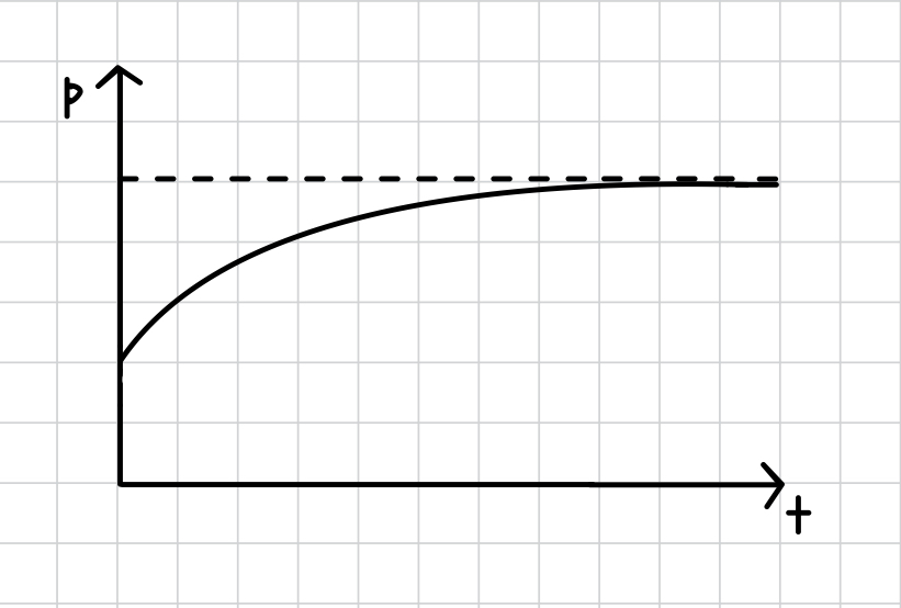
Population dynamics
This may represent, for example, a population with limited resources.
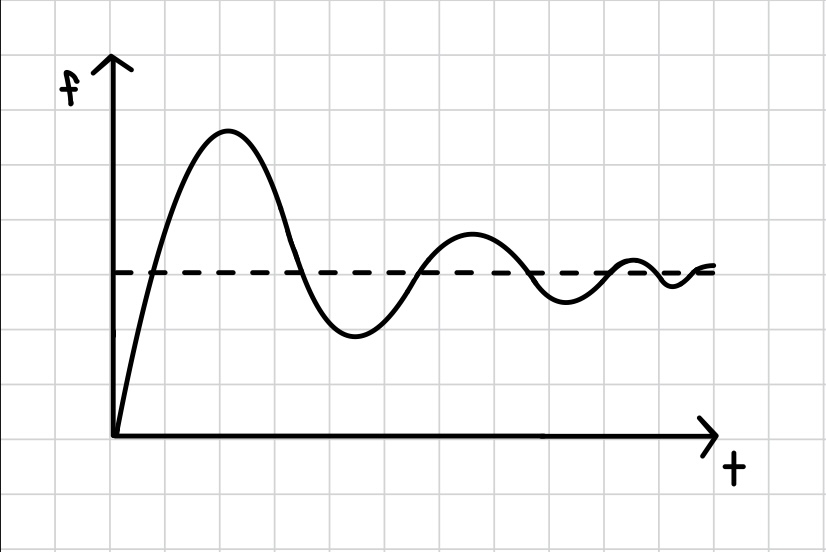
Proportional-integral control
This may represent, for example, the response of a servo or valve over time.
Limit at infinity
lim x → ∞ f ( x ) = L \lim_{x \to \infty} f(x) = L x → ∞ lim f ( x ) = L if for every ϵ > 0 \epsilon > 0 ϵ > 0 M such that for all x ,
if x > M x > M x > M ∣ f ( x ) − L ∣ < ϵ |f(x) - L| < \epsilon ∣ f ( x ) − L ∣ < ϵ
i.e., f gets close to L when x is “big”.
Some important limits at infinity:
lim x → ± ∞ k = k \displaystyle\lim_{x \to \pm\infty} k = k x → ± ∞ lim k = k
lim x → ± ∞ 1 x = 0 \displaystyle\lim_{x \to \pm\infty} \dfrac{1}{x} = 0 x → ± ∞ lim x 1 = 0
lim x → − ∞ e x = 0 \displaystyle\lim_{x \to -\infty} e^x = 0 x → − ∞ lim e x = 0
Other limit laws (sum, quotient, etc.) also hold at infinity! If function is
already in a convenient form, use known limits to evaluate unknown ones. For
example,
lim x → ∞ 5 + 1 x = lim x → ∞ 5 + lim x → ∞ 1 x = 5 + 0 = 5 \lim_{x \to \infty} 5 + \frac{1}{x} =
\lim_{x \to \infty} 5 + \lim_{x \to \infty} \frac{1}{x} =
5 + 0 = 5 x → ∞ lim 5 + x 1 = x → ∞ lim 5 + x → ∞ lim x 1 = 5 + 0 = 5 For rational functions f ( x ) = p ( x ) / q ( x ) f(x) = p(x) / q(x) f ( x ) = p ( x ) / q ( x ) x in
denominator:
lim x → − ∞ 11 x + 2 2 x 3 − 1 = lim x → − ∞ 11 x x 3 + 2 x 3 2 x 3 x 3 + 1 x 3 = 0 + 0 2 − 0 = 0 \lim_{x \to -\infty} \frac{11x + 2}{2x^3-1} =
\lim_{x \to -\infty} \frac{ \dfrac{11x}{x^3} + \dfrac{2}{x^3} }{ \dfrac{2x^3}{x^3} + \dfrac{1}{x^3}}
= \frac{0 + 0}{2 - 0} = 0 x → − ∞ lim 2 x 3 − 1 11 x + 2 = x → − ∞ lim x 3 2 x 3 + x 3 1 x 3 11 x + x 3 2 = 2 − 0 0 + 0 = 0 lim x → ∞ 5 x 2 + 8 x − 3 3 x 2 + 4 = lim x → ∞ 5 + 8 x − 3 x 2 3 + 2 x 2 = 5 + 0 − 0 3 − 0 = 5 3 \lim_{x \to \infty} \frac{5x^2+8x-3}{3x^2+4} =
\lim_{x \to \infty} \frac{ 5 + \dfrac{8}{x} - \dfrac{3}{x^2} }{ 3 + \dfrac{2}{x^2} } =
\frac{5+0-0}{3 - 0} = \frac{5}{3} x → ∞ lim 3 x 2 + 4 5 x 2 + 8 x − 3 = x → ∞ lim 3 + x 2 2 5 + x 8 − x 2 3 = 3 − 0 5 + 0 − 0 = 3 5 Not all functions have limits at infinity. Some “blow up”!
lim x → ∞ 2 x 2 − 3 7 x + 4 = lim x → ∞ 2 x − 3 x 7 + 4 x \lim_{x \to \infty} \frac{2x^2-3}{7x+4} = \lim_{x \to \infty} \frac{ 2x - \frac{3}{x} }{ 7 + \frac{4}{x} } x → ∞ lim 7 x + 4 2 x 2 − 3 = x → ∞ lim 7 + x 4 2 x − x 3 This limit does not exist. A helpful shortcut for rational polynomials: check
coefficients of highest powers in numerator and denominator!
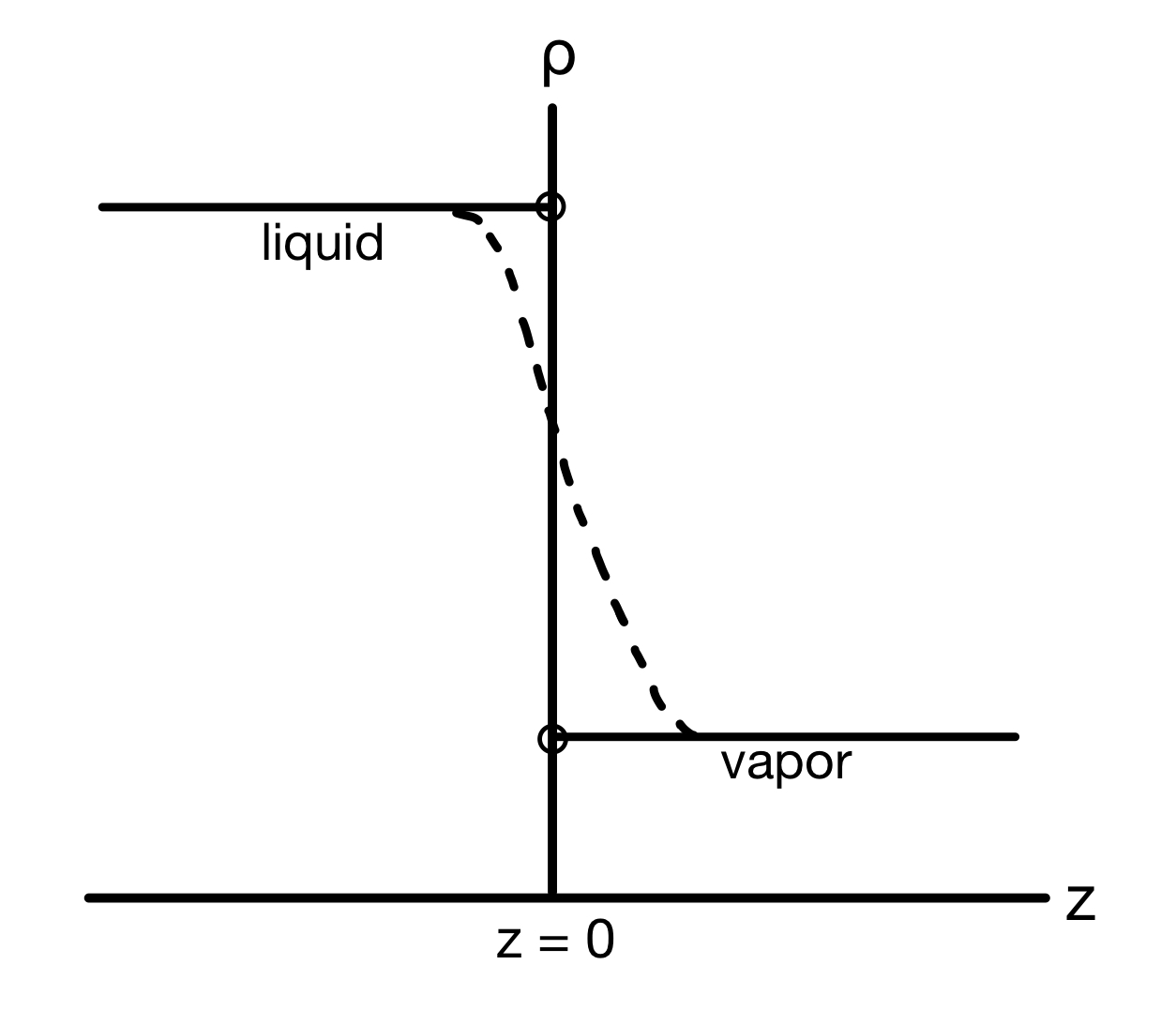
One-sided limits ¶ How do functions behave as you approach a point x 0 x_0 x 0
If the density as a function of distance from the interface is ρ ( z ) \rho(z) ρ ( z ) lim z → 0 − ρ ( z ) \lim_{z \to 0^-} \rho(z) lim z → 0 − ρ ( z ) lim z → 0 + ρ ( z ) \lim_{z \to 0^+} \rho(z) lim z → 0 + ρ ( z )
One-sided limit
If f is defined on the interval x 0 < x < b x_0 < x < b x 0 < x < b f ( x ) f(x) f ( x ) L L L x x x x 0 x_0 x 0 f f f L L L x 0 x_0 x 0
lim x → x 0 + f ( x ) = L \lim_{x \to x_0^+} f(x) = L x → x 0 + lim f ( x ) = L (This limit can also be written more formally in δ \delta δ ϵ \epsilon ϵ a < x < x 0 a < x < x_0 a < x < x 0
lim x → x 0 − f ( x ) = L \lim_{x \to x_0^-} f(x) = L x → x 0 − lim f ( x ) = L The two-sided limit exists if and only if both one-sided limits exist and have
the same value:
lim x → x 0 f ( x ) = L ⇔ lim x → x 0 + f ( x ) = lim x → x 0 − f ( x ) = L \lim_{x \to x_0} f(x) = L \Leftrightarrow
\lim_{x \to x_0^+} f(x) = \lim_{x \to x_0^-} f(x) = L x → x 0 lim f ( x ) = L ⇔ x → x 0 + lim f ( x ) = x → x 0 − lim f ( x ) = L For example, if
f ( x ) = ∣ x ∣ x = { − 1 , x < 0 1 , x > 0 f(x) = \frac{|x|}{x} = \begin{cases}
-1, & x<0\\
1, & x>0
\end{cases} f ( x ) = x ∣ x ∣ = { − 1 , 1 , x < 0 x > 0 We see that lim x → 0 + f ( x ) = 1 \lim_{x \to 0^+} f(x) = 1 lim x → 0 + f ( x ) = 1 lim x → 0 − f ( x ) = − 1 \lim_{x \to 0^-} f(x) = -1 lim x → 0 − f ( x ) = − 1 lim x → 0 f ( x ) \lim_{x \to 0} f(x) lim x → 0 f ( x )
Normal limit laws also still apply to one-sided limits:
lim x → − 2 + ( x x + 1 ) ( 2 x + 5 x 2 + x ) = ( − 2 − 2 + 1 ) ( − 4 + 5 4 − 2 ) = 1 \lim_{x \to -2^+} \left( \frac{x}{x+1} \right) \left( \frac{2x + 5}{x^2 + x} \right)
= \left( \frac{-2}{-2 + 1} \right) \left( \frac{-4 + 5}{4 - 2} \right) = 1 x → − 2 + lim ( x + 1 x ) ( x 2 + x 2 x + 5 ) = ( − 2 + 1 − 2 ) ( 4 − 2 − 4 + 5 ) = 1 However, be careful about which piece of the function applies:
lim x → − 2 − ( x + 3 ) ∣ x + 2 ∣ x + 2 = ( lim x → − 2 − x + 3 ) ( lim x → − 2 − ∣ x + 2 ∣ x + 2 ) = ( − 2 + 3 ) ( − 1 ) = − 1 \begin{align}
\lim_{x \to -2^-} (x + 3) \frac{|x + 2|}{x + 2}
&= \left( \lim_{x \to -2^-} x + 3 \right)
\left( \lim_{x \to -2^-} \frac{|x + 2|}{x + 2} \right) \\
&= (-2 + 3)(-1) = -1
\end{align} x → − 2 − lim ( x + 3 ) x + 2 ∣ x + 2∣ = ( x → − 2 − lim x + 3 ) ( x → − 2 − lim x + 2 ∣ x + 2∣ ) = ( − 2 + 3 ) ( − 1 ) = − 1 where we used the limit we already found of f ( x ) = ∣ x ∣ / x f(x) = |x|/x f ( x ) = ∣ x ∣/ x
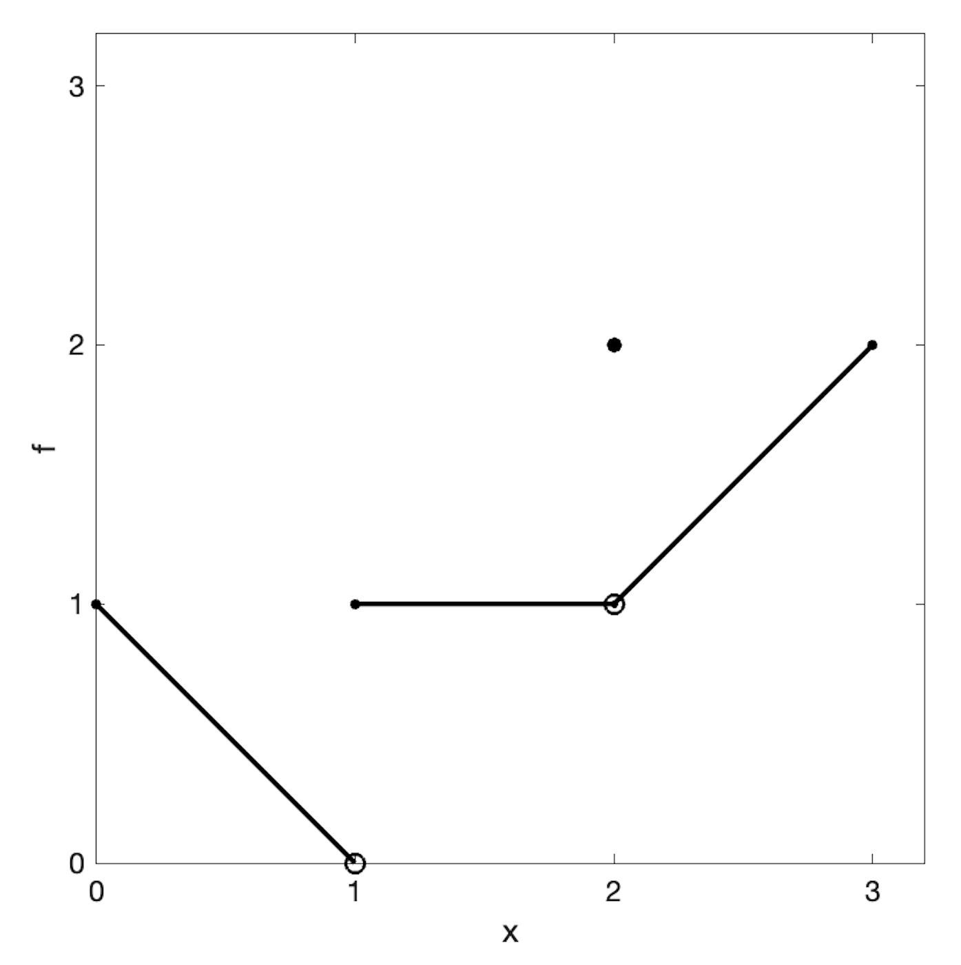
One-sided limit challenge ¶ Using
Find the limits at x = 1 x = 1 x = 1 x = 2 x = 2 x = 2
From the graph, lim x → 1 − f ( x ) = 0 \lim_{x \to 1^-} f(x) = 0 lim x → 1 − f ( x ) = 0 lim x → 1 + f ( x ) = 1 \lim_{x \to 1^+} f(x) = 1 lim x → 1 + f ( x ) = 1 lim x → 1 f ( x ) \lim_{x \to 1} f(x) lim x → 1 f ( x ) lim x → 2 − f ( x ) = 1 \lim_{x \to 2^-} f(x) = 1 lim x → 2 − f ( x ) = 1 lim x → 2 + f ( x ) = 1 \lim_{x \to 2^+} f(x) = 1 lim x → 2 + f ( x ) = 1 lim x → 2 f ( x ) = 1 \lim_{x \to 2} f(x) = 1 lim x → 2 f ( x ) = 1 f ( 2 ) = 2 f(2) = 2 f ( 2 ) = 2
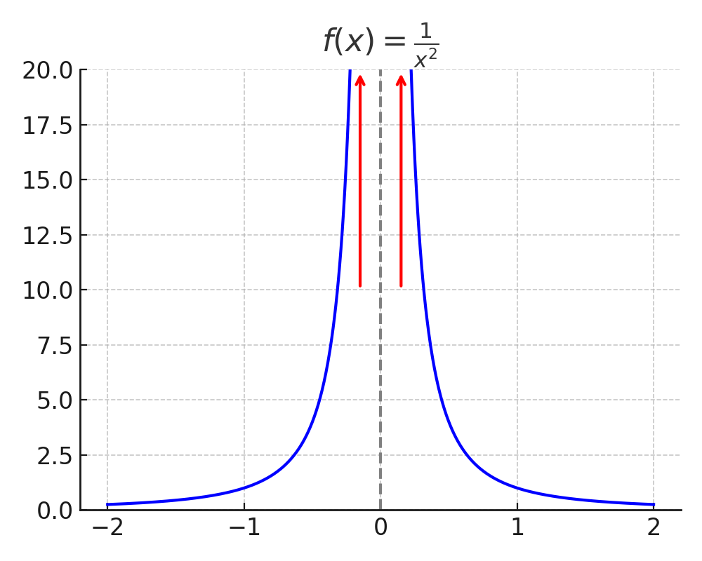
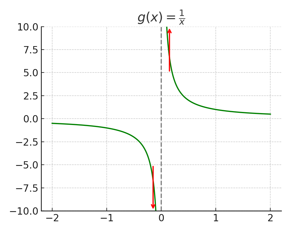
Infinite limits ¶ Some functions tend to ± ∞ \pm\infty ± ∞
f ( x ) = 1 / x 2 f(x) = 1/x^2 f ( x ) = 1/ x 2 Limit exists and is + ∞ +\infty + ∞
g ( x ) = 1 / x g(x) = 1/x g ( x ) = 1/ x Limit does not exist.
Infinite limits
f ( x ) f(x) f ( x ) ∞ \infty ∞ x approaches x 0 x_0 x 0
lim x → ∞ f ( x ) = ∞ \lim_{x\to\infty}f(x) = \infty x → ∞ lim f ( x ) = ∞ if for every real B there exists δ > 0 \delta > 0 δ > 0 x if
0 < ∣ x − x 0 ∣ < δ 0 < |x - x_0| < \delta 0 < ∣ x − x 0 ∣ < δ f ( x ) > f(x) > f ( x ) > − ∞ -\infty − ∞
This behavior can be used to define a vertical asymptote of a function:
L’Hôpital’s Rule ¶ L’Hôpital’s rule is a method that allows you to calculate limits of certain
indeterminate forms using derivatives.
L’Hôpital’s Rule
If lim x → a f ( x ) = lim x → a g ( x ) = 0 \lim_{x\to a} f(x) = \lim_{x \to a} g(x) = 0 lim x → a f ( x ) = lim x → a g ( x ) = 0 ± ∞ \pm \infty ± ∞
lim x → a f ( x ) g ( x ) = lim x → a f ′ ( x ) g ′ ( x ) \lim_{x\to a} \frac{f(x)}{g(x)} = \lim_{x\to a} \frac{f'(x)}{g'(x)} x → a lim g ( x ) f ( x ) = x → a lim g ′ ( x ) f ′ ( x ) This process can be repeated until the above situation no longer applies or
the limit is found not to exist.
Let’s work some examples:
The limits of the numerator and denominator are both zero, so:
lim x → 0 sin x x = lim x → 0 cos x 1 = 1 \lim_{x\to 0} \frac{\sin x}{x} = \lim_{x\to 0} \frac{\cos x}{1} = 1 x → 0 lim x sin x = x → 0 lim 1 cos x = 1 The limits of the numerator and denominator are both zero, so:
lim x → 0 x − sin x x 3 = lim x → 0 1 − cos x 3 x 2 = lim x → 0 sin x 6 x = 1 6 lim x → 0 sin x x = 1 6 \begin{align}
\lim_{x\to 0} \frac{x-\sin x}{x^3}
&= \lim_{x\to 0} \frac{1-\cos x}{3x^2} \\
&= \lim_{x\to 0} \frac{\sin x}{6x} \\
&= \frac{1}{6} \lim_{x\to 0} \frac{\sin x}{x} = \frac{1}{6}
\end{align} x → 0 lim x 3 x − sin x = x → 0 lim 3 x 2 1 − cos x = x → 0 lim 6 x sin x = 6 1 x → 0 lim x sin x = 6 1 where we used L’Hôpital’s rule twice, then used the result from the first
example.
The limits of the numerator and denominator are both ∞ \infty ∞
lim x → ∞ ln x 2 x = lim x → ∞ 1 / x 1 / x = lim x → ∞ 1 x = 0 \begin{align}
\lim_{x\to \infty} \frac{\ln x}{2\sqrt{x}}
&= \lim_{x\to \infty} \frac{1/x}{1/\sqrt{x}} \\
&= \lim_{x\to \infty} \frac{1}{\sqrt{x}} = 0
\end{align} x → ∞ lim 2 x ln x = x → ∞ lim 1/ x 1/ x = x → ∞ lim x 1 = 0 where the last limit is obtained by simplification.
The limits of the numerator and denominator are both ∞ \infty ∞
lim x → ∞ e x x 2 = lim x → ∞ e x 2 x = lim x → ∞ e x 2 = ∞ \begin{align}
\lim_{x\to \infty} \frac{e^x}{x^2}
&= \lim_{x\to \infty} \frac{e^x}{2x} \\
&= \lim_{x\to \infty} \frac{e^x}{2} = \infty
\end{align} x → ∞ lim x 2 e x = x → ∞ lim 2 x e x = x → ∞ lim 2 e x = ∞ Here, we used L’Hôpital’s rule twice, but then ultimately found that the
limit does not exist.
This limit is not in a form that’s immediately suitable for L’Hôpital’s rule,
but it can be made so.
lim x → ∞ x sin ( 1 / x ) = lim x → ∞ sin ( 1 / x ) 1 / x = lim x → ∞ cos ( 1 / x ) ( − 1 / x 2 ) − 1 / x 2 = lim x → ∞ cos ( 1 / x ) = 1 \begin{align}
\lim_{x\to \infty} x\sin(1/x)
&= \lim_{x\to \infty} \frac{\sin(1/x)}{1/x} \\
&= \lim_{x\to \infty} \frac{\cos(1/x)(-1/x^2)}{-1/x^2} \\
&= \lim_{x\to \infty} \cos(1/x) = 1
\end{align} x → ∞ lim x sin ( 1/ x ) = x → ∞ lim 1/ x sin ( 1/ x ) = x → ∞ lim − 1/ x 2 cos ( 1/ x ) ( − 1/ x 2 ) = x → ∞ lim cos ( 1/ x ) = 1 Another option in this case would be to substitute in y = 1 / x y = 1/x y = 1/ x y → 0 y \to 0 y → 0 x → ∞ x \to \infty x → ∞
lim y → 0 sin y y = 1 \lim_{y\to 0} \frac{\sin y}{y} = 1 y → 0 lim y sin y = 1 which we already solved!