4.3 Root finding methods

Fixed point iteration¶

Example: Fixed point iteration¶

Solve

First rearrange

Then, guess $x_0 = 0$ and set up a table:

At each iteration, $g(x_n)$ is used as the new $x_n$ until at $n = 5$, where $x_n = 0.6530 \approx 0.6528 = g(x_n)$.

Note that the choice of rearranging $f(x)$ is not unique, and some choices may be better than others. For example, convergence is only guaranteed when $|g'(x)| \le k < 1$ for all $x$ in an interval around the solution. Experience will guide your choice of rearrangement.

For example, to solve

One possible (but not obviously better) rearrangement is

Bisection search¶

We can apply this concept to find roots using the following procedure, called bisection search:

Example: Bisection search¶

Solve

Start with $a_0 = 0$ and $b_0 = 1$, then make a table to implement the procedure:

When $n=0$, $f(x_0)$ > 0 so $a_1$ = $x_0$. Then, when $n=1$, $f(x_1)$ < 0 so $b_2$ = $x_1$. We continue this procedure until convergence.

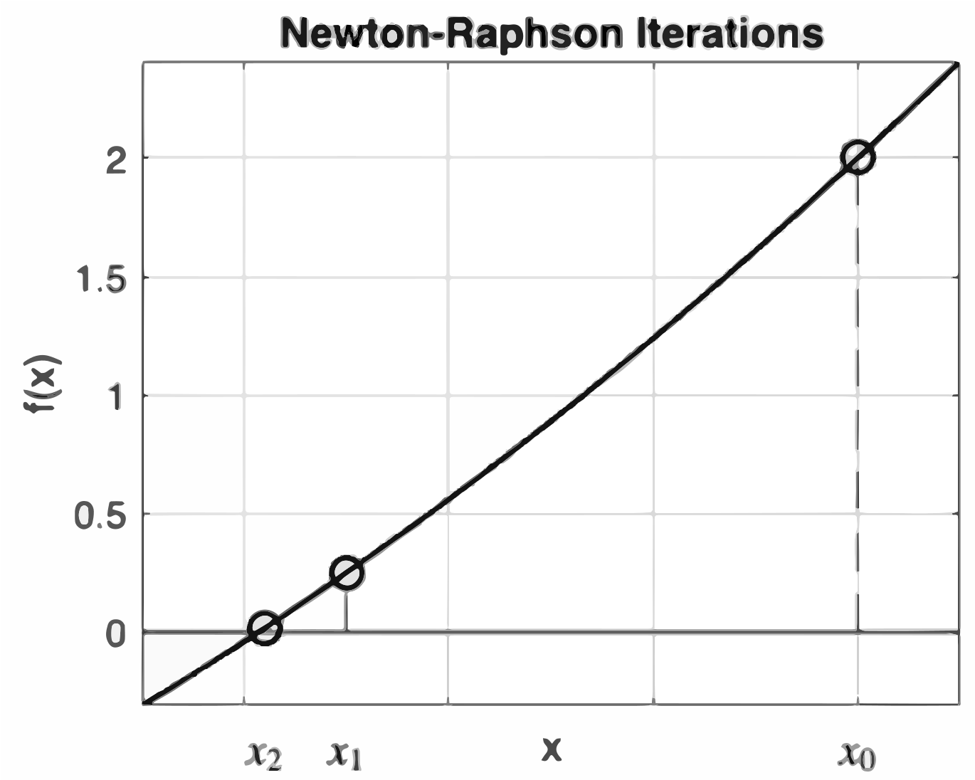
Newton-Raphson method¶

Although we cannot immediately solve the nonlinear equation $f(x) = 0$, we can first linearize it, then solve the linear problem.

Iterating this process gives the Newton-Raphson method of root finding

Note that this method can converge much more rapidly than the fixed-point or bisection methods. However, it will fail if $f'(x_n) = 0$.

Example 1: Newton-Raphson method¶

Solve $x^2 = 2$.

We can rewrite this as $f(x) = x^2-2 = 0$. We will also evaluate the derivative $f'(x) = 2x$. Let the initial guess be $x_0 = 1$.

This is close to the known value of $\sqrt{2}$!

Example 2: Newton-Raphson method¶

Solve $e^{-x^2} - x = 0$.

We define $f(x) = e^{-x^2} - x$ and calculate $f'(x) = -2x e^{-x^2} - 1$. We choose an initial guess $x_0 = 0$.

Note the rapid convergence compared to the methods above!

Skill builder problems¶

Solve

to 3 significant figures by: