3.1 Matrices and vectors
Matrices and vectors are convenient tools for representing linear systems with
compact notation that can be processed by a computer.
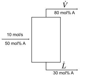
For example, say you are analyzing the molar flow rates resulting from a flash
distillation process.
The steady-state mole balances for the total process and component A are
10 = L ˙ + V ˙ 5 = 0.3 L ˙ + 0.8 V ˙ \begin{align}
10 &= \dot L + \dot V \\
5 &= 0.3 \dot L + 0.8 \dot V
\end{align} 10 5 = L ˙ + V ˙ = 0.3 L ˙ + 0.8 V ˙ These equations can equivalently be represented using matrices and vectors as
[ 10 5 ] = [ 1 1 0.3 0.8 ] [ L ˙ V ˙ ] \begin{bmatrix} 10 \\ 5 \end{bmatrix} =
\begin{bmatrix} 1 & 1 \\ 0.3 & 0.8 \end{bmatrix}
\begin{bmatrix} \dot L \\ \dot V \end{bmatrix} [ 10 5 ] = [ 1 0.3 1 0.8 ] [ L ˙ V ˙ ] We will learn why these representations are equivalent shortly. Importantly,
because our mole balances can be written in this way, they are a system of
linear equations that can be solved using techniques of linear algebra.
Definition ¶ A matrix is a rectangular array of quantities, which we call its elements ,
that are laid out in horizontal rows and vertical columns . We will typically
denote a matrix by a bold, capital letter such as A .
A = [ 0.3 1 − 5 0 − 0.2 16 ] \vv{A} = \begin{bmatrix} 0.3 & 1 & -5 \\ 0 & -0.2 & 16 \end{bmatrix} A = [ 0.3 0 1 − 0.2 − 5 16 ] An m x n matrix has m rows and n columns. A is a 2 x 3 matrix. We
will sometimes refer to elements of a matrix by their row and column
A = [ A 11 A 12 A 13 A 21 A 22 A 23 ] \vv{A} = \begin{bmatrix} A_{11} & A_{12} &
A_{13} \\ A_{21} & A_{22} & A_{23} \end{bmatrix} A = [ A 11 A 21 A 12 A 22 A 13 A 23 ] For example, A 12 = 1 A_{12} = 1 A 12 = 1 A 23 = 16 A_{23} = 16 A 23 = 16 A given above.
A vector is a matrix with either one column (a column vector ) or one row (a
row vector ). We will typically denote a vector by a bold, lowercase letter
such as b
b = [ 1 2 ] c = [ − 1 0 1 ] \vv{b} = \begin{bmatrix} 1 \\ 2 \end{bmatrix} \qquad
\vv{c} = \begin{bmatrix} -1 & 0 & 1 \end{bmatrix} b = [ 1 2 ] c = [ − 1 0 1 ] b is a 2-element column vector that is also a 2 x 1 matrix, while c is a
3-element row vector that is also a 1 x 3 matrix. When referring to elements of
a vector, it typical to only use one index
b = [ b 1 b 2 ] c = [ c 1 c 2 c 3 ] \vv{b} = \begin{bmatrix} b_1 \\ b_2 \end{bmatrix} \qquad
\vv{c} = \begin{bmatrix} c_1 & c_2 & c_3 \end{bmatrix} b = [ b 1 b 2 ] c = [ c 1 c 2 c 3 ] For b and c given above, b 2 = 2 b_2 = 2 b 2 = 2 c 2 = 0 c_2 = 0 c 2 = 0
There are some other types of “special” matrices.
Square matrix : a matrix with equal numbers of rows and columns (an n x n
matrix).
[ 1 2 4 3 ] \begin{bmatrix} 1 & 2 \\ 4 & 3 \end{bmatrix} [ 1 4 2 3 ] Diagonal matrix : a square matrix with nonzero entries only for the elements
on the diagonal, A i i A_{ii} A ii i = 1 , . . . , n i = 1, ..., n i = 1 , ... , n
[ 1 0 0 3 ] \begin{bmatrix} 1 & 0 \\ 0 & 3 \end{bmatrix} [ 1 0 0 3 ] Upper triangular matrix : a square matrix with nonzero entries only on the
diagonal or above, A i j A_{ij} A ij i = 1 , . . . , n i = 1, ..., n i = 1 , ... , n j ≥ i j \ge i j ≥ i A i i A_{ii} A ii
[ 1 2 0 3 ] \begin{bmatrix} 1 & 2 \\ 0 & 3 \end{bmatrix} [ 1 0 2 3 ] Lower triangular matrix : a square matrix with nonzero entries only on the
diagonal or below, A i j A_{ij} A ij i = 1 , . . . , n i = 1, ..., n i = 1 , ... , n j ≤ i j \le i j ≤ i
[ 1 0 4 3 ] \begin{bmatrix} 1 & 0 \\ 4 & 3 \end{bmatrix} [ 1 4 0 3 ] Identity matrix : a diagonal matrix of ones, typically denoted I .
[ 1 0 0 1 ] \begin{bmatrix} 1 & 0 \\ 0 & 1 \end{bmatrix} [ 1 0 0 1 ] There are several other types of special matrices, but we will leave those for a
longer course on linear algebra!
Addition and scalar multiplication ¶ Equality : A = B \vv{A} = \vv{B} A = B A and B have the same
size and all their corresponding elements are equal.
Addition : C = A + B \vv{C} = \vv{A} + \vv{B} C = A + B A and B have the
samesize. Then, the matrix elements are added element-wise:
C i j = A i j + B i j C_{ij} = A_{ij} + B_{ij} C ij = A ij + B ij Example:
[ 5 − 1 0 3 1 0 ] + [ 1 5 3 3 2 2 ] = [ − 4 6 3 0 1 2 ] \begin{bmatrix} 5 & -1 & 0 \\ 3 & 1 & 0 \end{bmatrix} +
\begin{bmatrix} 1 & 5 & 3 \\ 3 & 2 & 2 \end{bmatrix} =
\begin{bmatrix} -4 & 6 & 3 \\ 0 & 1 & 2 \end{bmatrix} [ 5 3 − 1 1 0 0 ] + [ 1 3 5 2 3 2 ] = [ − 4 0 6 1 3 2 ] Scalar multiplication : B = k A \vv{B} = k\vv{A} B = k A A
by k :
B i j = k A i j B_{ij} = kA_{ij} B ij = k A ij Example:
− 2 [ 1 0 0 − 2 ] = [ − 2 × 1 − 2 × 0 − 2 × 0 − 2 × 4 ] = [ − 2 0 0 4 ] -2 \begin{bmatrix} 1 & 0 \\ 0 & -2 \end{bmatrix}
= \begin{bmatrix} -2 \times 1 & -2 \times 0 \\ -2 \times 0 & -2 \times 4 \end{bmatrix}
= \begin{bmatrix} -2 & 0 \\ 0 & 4 \end{bmatrix} − 2 [ 1 0 0 − 2 ] = [ − 2 × 1 − 2 × 0 − 2 × 0 − 2 × 4 ] = [ − 2 0 0 4 ] Subtraction : same as addition of negative
C = A − B = A + ( − B ) \vv{C} = \vv{A} - \vv{B} = \vv{A} + (-\vv{B}) C = A − B = A + ( − B )
C i j = A i j − B i j C_{ij} = A_{ij} - B_{ij} C ij = A ij − B ij For example, given
A = [ − 1 2 0 5 ] B = [ 1 0 0 1 ] \vv{A} = \begin{bmatrix} -1 & 2 \\ 0 & 5 \end{bmatrix} \qquad
\vv{B} = \begin{bmatrix} 1 & 0 \\ 0 & 1 \end{bmatrix} A = [ − 1 0 2 5 ] B = [ 1 0 0 1 ] Compute 2 A − B 2\vv{A} - \vv{B} 2 A − B
2 A − B = 2 [ − 1 2 0 5 ] − [ 1 0 0 1 ] = [ − 2 4 0 10 ] − [ 1 0 0 1 ] = [ − 3 4 0 9 ] \begin{align}
2\vv{A}-\vv{B} &= 2 \begin{bmatrix} -1 & 2 \\ 0 & 5 \end{bmatrix} -
\begin{bmatrix} 1 & 0 \\ 0 & 1 \end{bmatrix} \\
&= \begin{bmatrix} -2 & 4 \\ 0 & 10 \end{bmatrix} -
\begin{bmatrix} 1 & 0 \\ 0 & 1 \end{bmatrix} \\
&= \begin{bmatrix} -3 & 4 \\ 0 & 9 \end{bmatrix}
\end{align} 2 A − B = 2 [ − 1 0 2 5 ] − [ 1 0 0 1 ] = [ − 2 0 4 10 ] − [ 1 0 0 1 ] = [ − 3 0 4 9 ] Matrix multiplication ¶ C = AB is defined if A has the same number of columns as B has
rows. If A is m x p and B is p x n , C is m x n and its
elements are
C i j = ∑ k = 1 p A i k B k j C_{ij} = \sum_{k=1}^p A_{ik} B_{kj} C ij = k = 1 ∑ p A ik B kj Example:
[ 3 5 4 0 − 6 − 3 ] [ 2 − 2 5 0 ] = [ 3 × 2 + 5 × 5 3 × − 2 + 5 × 0 4 × 2 + 0 × 5 4 × − 2 + 0 × 0 − 6 × 2 + − 3 × 5 − 6 × − 2 + − 3 × 0 ] = [ 31 − 6 8 − 8 − 27 12 ] \begin{align}
\begin{bmatrix} 3 & 5 \\ 4 & 0 \\ -6 & -3 \end{bmatrix}
\begin{bmatrix} 2 & -2 \\ 5 & 0 \end{bmatrix}
&= \begin{bmatrix} 3\times2 + 5\times5 & 3\times-2 + 5\times0 \\
4\times2 + 0\times5 & 4\times-2 + 0\times0 \\
-6\times2 + -3\times5 & -6\times-2 + -3\times0 \end{bmatrix} \\
&= \begin{bmatrix} 31 & -6 \\ 8 & -8 \\ -27 & 12 \end{bmatrix}
\end{align} ⎣ ⎡ 3 4 − 6 5 0 − 3 ⎦ ⎤ [ 2 5 − 2 0 ] = ⎣ ⎡ 3 × 2 + 5 × 5 4 × 2 + 0 × 5 − 6 × 2 + − 3 × 5 3 × − 2 + 5 × 0 4 × − 2 + 0 × 0 − 6 × − 2 + − 3 × 0 ⎦ ⎤ = ⎣ ⎡ 31 8 − 27 − 6 − 8 12 ⎦ ⎤ Multiplying with a vector works the same!
[ 3 5 4 0 − 6 − 3 ] [ 1 2 ] = [ 3 × 1 + 5 × 2 4 × 1 + 0 × 2 − 6 × 1 + − 3 × 2 ] = [ 8 4 − 12 ] \begin{align}
\begin{bmatrix} 3 & 5 \\ 4 & 0 \\ -6 & -3 \end{bmatrix}
\begin{bmatrix} 1 \\ 2 \end{bmatrix}
&= \begin{bmatrix} 3 \times 1 + 5 \times 2 \\
4 \times 1 + 0 \times 2 \\
-6 \times 1 + -3 \times 2
\end{bmatrix} \\
&= \begin{bmatrix} 8 \\ 4 \\ -12 \end{bmatrix}
\end{align} ⎣ ⎡ 3 4 − 6 5 0 − 3 ⎦ ⎤ [ 1 2 ] = ⎣ ⎡ 3 × 1 + 5 × 2 4 × 1 + 0 × 2 − 6 × 1 + − 3 × 2 ⎦ ⎤ = ⎣ ⎡ 8 4 − 12 ⎦ ⎤ Transpose ¶ A T \vv{A}^{\rm T} A T A , and its elements are obtained by
“flipping” the rows and columns:
A i j T = A j i A_{ij}^{\rm T} = A_{ji} A ij T = A ji Example:
[ 1 2 4 3 ] T = [ 1 4 2 3 ] \begin{bmatrix} 1 & 2 \\ 4 & 3 \end{bmatrix}^{\rm T} =
\begin{bmatrix} 1 & 4 \\ 2 & 3 \end{bmatrix} [ 1 4 2 3 ] T = [ 1 2 4 3 ] A matrix is called symmetric if A T = A \vv{A}^{\rm T} = \vv{A} A T = A
Rules for transposition
( A T ) T = A (\vv{A}^{\rm T})^{\rm T} = \vv{A} ( A T ) T = A
( A + B ) T = A T + B T (\vv{A} + \vv{B})^{\rm T} = \vv{A}^{\rm T} + \vv{B}^{\rm T} ( A + B ) T = A T + B T
( A B ) T = B T + A T (\vv{A}\vv{B})^{\rm T} = \vv{B}^{\rm T} + \vv{A}^{\rm T} ( AB ) T = B T + A T
( k A ) T = k A T (k \vv{A})^{\rm T} = k\vv{A}^{\rm T} ( k A ) T = k A T
Skill builder problems ¶ Given the matrices:
A = [ 0 2 2 4 1 3 ] B = [ 0 2 1 2 4 3 ] C = [ 3 0 4 − 1 2 2 6 5 − 4 ] D = [ 0 − 5 − 3 − 5 2 4 − 3 4 0 ] \vv{A} = \begin{bmatrix} 0 & 2 \\ 2 & 4 \\ 1 & 3 \\ \end{bmatrix}
\quad
\vv{B} = \begin{bmatrix} 0 & 2 &1 \\ 2 & 4 & 3 \end{bmatrix}
\quad
\vv{C} = \begin{bmatrix} 3 & 0 & 4 \\ -1 & 2 & 2 \\ 6 & 5 & -4 \end{bmatrix}
\quad
\vv{D} = \begin{bmatrix} 0 & -5 & -3 \\ -5 & 2 & 4 \\ -3 & 4 & 0 \end{bmatrix} A = ⎣ ⎡ 0 2 1 2 4 3 ⎦ ⎤ B = [ 0 2 2 4 1 3 ] C = ⎣ ⎡ 3 − 1 6 0 2 5 4 2 − 4 ⎦ ⎤ D = ⎣ ⎡ 0 − 5 − 3 − 5 2 4 − 3 4 0 ⎦ ⎤ and vectors:
a = [ 1 3 ] b = [ 0 2 ] c = [ 2 0 − 1 ] \vv{a} = \begin{bmatrix} 1 \\ 3 \end{bmatrix}
\quad
\vv{b} = \begin{bmatrix} 0 & 2 \end{bmatrix}
\quad
\vv{c} = \begin{bmatrix} 2 \\ 0 \\ -1 \end{bmatrix} a = [ 1 3 ] b = [ 0 2 ] c = ⎣ ⎡ 2 0 − 1 ⎦ ⎤ Compute the following or explain why it is undefined.
2 A = [ 2 ⋅ 0 2 ⋅ 2 2 ⋅ 2 2 ⋅ 4 2 ⋅ 1 2 ⋅ 3 ] = [ 0 4 4 8 2 6 ] 2\vv{A}
= \begin{bmatrix}
2 \cdot 0 & 2 \cdot 2 \\
2 \cdot 2 & 2 \cdot 4 \\
2 \cdot 1 & 2 \cdot 3 \end{bmatrix}
= \begin{bmatrix} 0 & 4 \\ 4 & 8 \\ 2 & 6 \end{bmatrix} 2 A = ⎣ ⎡ 2 ⋅ 0 2 ⋅ 2 2 ⋅ 1 2 ⋅ 2 2 ⋅ 4 2 ⋅ 3 ⎦ ⎤ = ⎣ ⎡ 0 4 2 4 8 6 ⎦ ⎤ Undefined because the shape of A (3×2) is different from the shape of
B (2×3).
A T + B = [ 0 2 1 2 4 3 ] + [ 0 2 1 2 4 3 ] = [ 0 + 0 2 + 2 1 + 1 2 + 2 4 + 4 3 + 3 ] = [ 0 4 2 4 8 6 ] \begin{align}
\vv{A}^{\rm T} + \vv{B}
&= \begin{bmatrix} 0 & 2 & 1 \\ 2 & 4 & 3 \end{bmatrix}
+ \begin{bmatrix} 0 & 2 & 1\\ 2 & 4 & 3 \end{bmatrix} \\
&= \begin{bmatrix} 0+0 & 2+2 & 1+1 \\ 2+2 & 4+4 & 3+3 \end{bmatrix} \\
&= \begin{bmatrix} 0 & 4 & 2 \\ 4 & 8 & 6 \end{bmatrix}
\end{align} A T + B = [ 0 2 2 4 1 3 ] + [ 0 2 2 4 1 3 ] = [ 0 + 0 2 + 2 2 + 2 4 + 4 1 + 1 3 + 3 ] = [ 0 4 4 8 2 6 ] (or, A T = B \vv{A}^{\rm T} = \vv{B} A T = B A T + B = 2 B \vv{A}^{\rm T} + \vv{B} = 2\vv{B} A T + B = 2 B
C − D = [ 3 − 0 0 − ( − 5 ) 4 − ( − 3 ) − 1 − ( − 5 ) 2 − 2 2 − 4 6 − ( − 3 ) 5 − 4 − 4 − 0 ] = [ 3 5 7 4 0 − 2 9 1 − 4 ] \begin{align}
\vv{C} -\vv{D}
&= \begin{bmatrix}
3-0 & 0-(-5) & 4-(-3) \\
-1-(-5) & 2-2 & 2-4 \\
6-(-3) & 5-4 & -4-0 \end{bmatrix} \\
&= \begin{bmatrix} 3 & 5 & 7 \\ 4 & 0 & -2 \\ 9 & 1 & -4 \end{bmatrix}
\end{align} C − D = ⎣ ⎡ 3 − 0 − 1 − ( − 5 ) 6 − ( − 3 ) 0 − ( − 5 ) 2 − 2 5 − 4 4 − ( − 3 ) 2 − 4 − 4 − 0 ⎦ ⎤ = ⎣ ⎡ 3 4 9 5 0 1 7 − 2 − 4 ⎦ ⎤ A a = [ 0 ⋅ 1 + 2 ⋅ 3 2 ⋅ 1 + 4 ⋅ 3 1 ⋅ 1 + 3 ⋅ 3 ] = [ 6 14 10 ] \begin{align}
\vv{Aa}
&= \begin{bmatrix}
0 \cdot 1 + 2 \cdot 3 \\
2 \cdot 1 + 4 \cdot 3 \\
1 \cdot 1 + 3 \cdot 3 \end{bmatrix} \\
&= \begin{bmatrix} 6 \\ 14 \\ 10 \end{bmatrix}
\end{align} Aa = ⎣ ⎡ 0 ⋅ 1 + 2 ⋅ 3 2 ⋅ 1 + 4 ⋅ 3 1 ⋅ 1 + 3 ⋅ 3 ⎦ ⎤ = ⎣ ⎡ 6 14 10 ⎦ ⎤ Undefined because A has 2 columns but b has 1 row.
Undefined because A has 2 columns but c has 3 rows.
B c = [ 0 ⋅ 2 + 2 ⋅ 0 + 1 ⋅ − 1 2 ⋅ 2 + 4 ⋅ 0 + 3 ⋅ − 1 ] = [ − 1 1 ] \begin{align}
\vv{Bc}
&= \begin{bmatrix}
0 \cdot 2 + 2 \cdot 0 + 1 \cdot -1 \\
2 \cdot 2 + 4 \cdot 0 + 3 \cdot -1 \end{bmatrix} \\
&= \begin{bmatrix} -1 \\ 1 \end{bmatrix}
\end{align} Bc = [ 0 ⋅ 2 + 2 ⋅ 0 + 1 ⋅ − 1 2 ⋅ 2 + 4 ⋅ 0 + 3 ⋅ − 1 ] = [ − 1 1 ] c T A = [ 0 2 − 1 ] [ 0 2 2 4 1 3 ] = [ 2 ⋅ 0 + 0 ⋅ 2 + − 1 ⋅ 1 2 ⋅ 2 + 0 ⋅ 4 ⋅ − 1 ⋅ 3 ] = [ − 1 1 ] \begin{align}
\vv{c}^{\rm T} \vv{A}
&= \begin{bmatrix} 0 & 2 & -1\end{bmatrix}
\begin{bmatrix} 0 & 2 \\ 2 & 4 \\ 1 &3 \end{bmatrix} \\
&= \begin{bmatrix}
2 \cdot 0 + 0 \cdot 2 + -1 \cdot 1 &
2 \cdot 2 + 0 \cdot 4 \cdot -1 \cdot 3 \end{bmatrix} \\
&= \begin{bmatrix} -1 & 1 \end{bmatrix}
\end{align} c T A = [ 0 2 − 1 ] ⎣ ⎡ 0 2 1 2 4 3 ⎦ ⎤ = [ 2 ⋅ 0 + 0 ⋅ 2 + − 1 ⋅ 1 2 ⋅ 2 + 0 ⋅ 4 ⋅ − 1 ⋅ 3 ] = [ − 1 1 ]