3.3 Gauss–Jordan elimination

To solve a system of linear equations like

Note that the second equation is easily solved for $x_2 = -2$, which can be substituted in the first equation to give $x_1 = (2-5x_2)/2 = 6$. If we can bring systems so that one variable is isolated, we can work backwards to solve the others! How do we do this systematically for equations?

Because of 2 and 3, we can also add a multiple of one equation to another.

For example, suppose we instead started with the equations

Adding twice the first equation to the second equation gives $13 x_2 = -26$, from which we were able solve before!

Procedure¶

This process can be tedious, particularly when there are more variables and equations. Matrices provide a systematic approach to both performing elementary operations to isolate variables, as well as to carry out subsequent substitution. This entire procedure is called Gauss-Jordan elimination with backsubstitution.

1. Rewrite the equations as $\vv{A}\vv{x} = \vv{b}$ using a matrix and vectors

   $$\begin{bmatrix}2 5 \\ -4 3\end{bmatrix} \begin{bmatrix}x_1 \\ x_2\end{bmatrix} = \begin{bmatrix}2 \\ -30\end{bmatrix}$$

   (3)

2. Form the “augmented” matrix $[\vv{A} \vv{b}]$

   $$\mathbf{A} = \begin{bmatrix} 2 & 5 & 2\\ -4 & 3 & -30\end{bmatrix}$$

   (4)

3. Perform elementary operations on rows to create “pivot” points in each row. The goal is to get a number on the diagonals and zeros below. It is OK to have a zero on the diagonal if there are no nonzero values underneath it.

   $$\begin{bmatrix} 2 & 5 & 2 \\ -4 & 3 & -30 \end{bmatrix} \begin{matrix}\vphantom{R_1} \\ +2 R_1 \end{matrix} \to \begin{bmatrix} 2 & 5 & 2 \\ 0 & 13 & -26 \end{bmatrix}$$

   (5)

   Here, we noted that we added twice Row 1 to Row 2 to eliminate the 4 under the first pivot point 2.

4. When you reach the bottom row, check there are no rows of zeros with a nonzero last column. This would be equivalent to a false equation (like $0=1$), meaning there is no solution and no further work is needed.

5. Work back up to turn pivot points into ones and get zeros above in each column

   $$\begin{align} \begin{bmatrix} 2 & 5 & 2 \\ 0 & 13 & -26 \end{bmatrix} \begin{matrix}\vphantom{R_1} \\ \div 13 \end{matrix} &\to \begin{bmatrix} 2 & 5 & 2 \\ 0 & 1 & -2 \end{bmatrix} \begin{matrix}-5 R_2 \\ \vphantom{R_2}\end{matrix} \\ &\to \begin{bmatrix} 2 & 0 & 12 \\ 0 & 1 & -2 \end{bmatrix} \begin{matrix}\div 2 \\ \vphantom{R_2}\end{matrix} \\ &\to \begin{bmatrix} 1 & 0 & 6 \\ 0 & 1 & -2 \end{bmatrix} \end{align}$$

   (6)

6. The solution comes from reexpressing the augmented matrix as $\vv{A} \vv{x} = \vv{b}$.

   $$\begin{bmatrix} 1 & 0 \\ 0 & 1 \end{bmatrix} \begin{bmatrix} x_1 \\ x_2 \end{bmatrix} = \begin{bmatrix} 6 \\ -2 \end{bmatrix}$$

   (7)

   Or, $x_1 = 6$ and $x_2 = -2$.

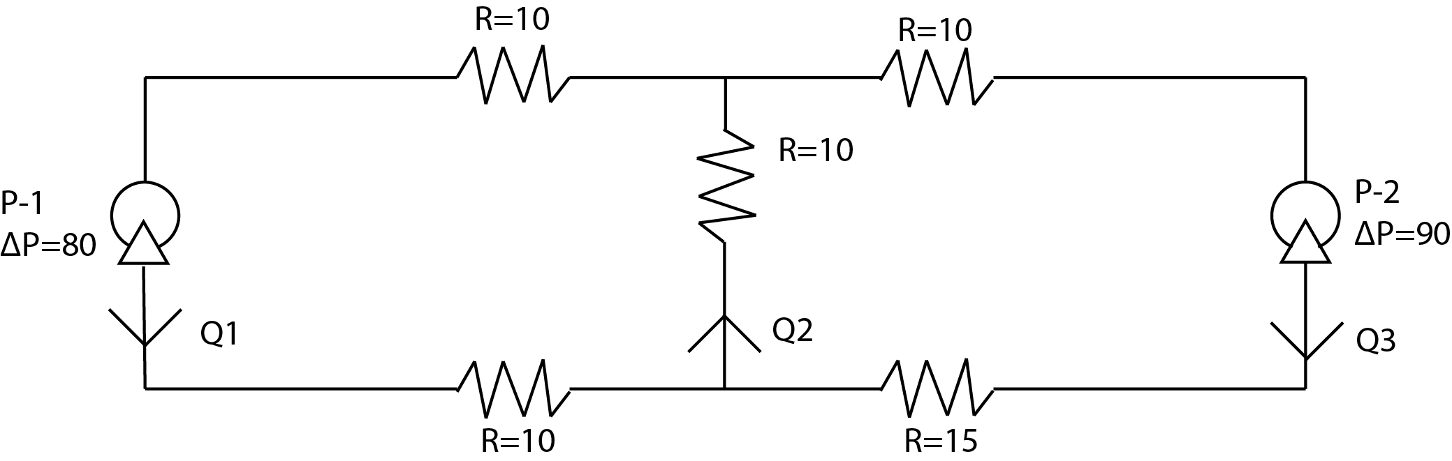
Example: Pump circuit¶

Incompressible flow can be written analogous to an electrical circuit as

where $\Delta P$ is the pressure change, R is the resistance, and Q is the volumetric flow rate. For the following pump “circuit”:

The pressure and mass balances for the nodes and loop give:

Find $Q_1$, $Q_2$, and $Q_3$.

First, rearrange the equations into consistent linear form:

Then, rewrite using matrix representation:

Now, perform Gauss-Jordan elimination steps to solve for the unknown flow rates. We form the augmented matrix, then use Row 1 to eliminate values in Rows 2 and 3:

Row 2 is all zeros because it was a redundant equation to Row 1. Swap Rows 2 and 4, then use the new Row 2 to eliminate value in Row 3:

Normalize Row 3 (divide by -95), then eliminate values above in Column 3:

Normalize Row 2 (divide by 10), then eliminate values above in Column 2:

Turning back into an equivalent system of equations gives the final solution, $Q_1 = 2$, $Q_2 = 4$, and $Q_3 = 2$.

Number of solutions¶

The number of solutions for the system of linear equations can be determined from the row-reduced augmented matrix.

• There is no solution if there is a row of zeroes with a nonzero last column.

  $$\begin{align} \begin{bmatrix} 3 & 2 & 1 & 3 \\ 2 & 1 & 1 & 0 \\ 6 & 2 & 4 & 6 \end{bmatrix} \begin{matrix}\vphantom{R_1} \\ -(2/3) R_1 \\ -2 R_1 \end{matrix} &\to \begin{bmatrix} 3 & 2 & 1 & 3 \\ 0 & -1/3 & 1/3 & -2 \\ 0 & -2 & 2 & 0 \end{bmatrix} \begin{matrix}\vphantom{R_1} \\ \times -3 \\ \div 2\end{matrix} \\ &\to \begin{bmatrix} 3 & 2 & 1 & 3 \\ 0 & 1 & -1 & 6 \\ 0 & -1 & 1 & 0 \end{bmatrix} \begin{matrix}\vphantom{R_1} \\ \vphantom{R_2} \\ +R_2 \end{matrix} \\ &\to \begin{bmatrix} 3 & 2 & 1 & 3 \\ 0 & 1 & -1 & 6 \\ 0 & 0 & 0 & 12 \end{bmatrix} \end{align}$$

  (16)

  Since the last row is equivalent to $0 = 12$, there is a false equation and the system has no solution.

• There is one solution if there is one pivot for each unknown.

  $$\begin{align} \begin{bmatrix} 3 & 2 & 1 & 3 \\ 2 & 1 & 1 & 0 \\ 6 & 2 & 5 & 6 \end{bmatrix} \begin{matrix}\vphantom{R_1} \\ -(2/3) R_1 \\ -2 R_1 \end{matrix} &\to \begin{bmatrix} 3 & 2 & 1 & 3 \\ 0 & -1/3 & 1/3 & -2 \\ 0 & -2 & 3 & 0 \end{bmatrix} \begin{matrix}\vphantom{R_1} \\ \times -3 \\ \vphantom{R_3} \end{matrix} \\ &\to \begin{bmatrix} 3 & 2 & 1 & 3 \\ 0 & 1 & -1 & 6 \\ 0 & -2 & 3 & 0 \end{bmatrix} \begin{matrix}\vphantom{R_1} \\ \vphantom{R_2} \\ +2 R_2 \end{matrix} \\ &\to \begin{bmatrix} 3 & 2 & 1 & 3 \\ 0 & 1 & -1 & 6 \\ 0 & 0 & 1 & 12 \end{bmatrix} \begin{matrix} -R_3 \\ +R_3 \\ \vphantom{R_3} \end{matrix} \\ &\to \begin{bmatrix} 3 & 2 & 0 & -9 \\ 0 & 1 & 0 & 18 \\ 0 & 0 & 1 & 12 \end{bmatrix} \begin{matrix} -2R_2 \\ \vphantom{R_3} \end{matrix} \\ &\to \begin{bmatrix} 3 & 0 & 0 & -45 \\ 0 & 1 & 0 & 18 \\ 0 & 0 & 1 & 12 \end{bmatrix} \begin{matrix} \div 3 \\ \vphantom{R_3} \end{matrix} \\ &\to \begin{bmatrix} 1 & 0 & 0 & -15 \\ 0 & 1 & 0 & 18 \\ 0 & 0 & 1 & 12 \end{bmatrix} \end{align}$$

  (17)

  There are 3 pivot points and 3 unknowns, the solution is $x_1 = -15$, $x_2 = 18$, and $x_3 = 12$.

• There are infinitely many solutions if there are fewer pivots than unknowns.

  $$\begin{align} \begin{bmatrix} 3 & 2 & 1 & 3 \\ 2 & 1 & 1 & 0 \\ 6 & 2 & 4 & -6 \end{bmatrix} \begin{matrix}\vphantom{R_1} \\ -(2/3) R_1 \\ -2 R_1 \end{matrix} &\to \begin{bmatrix} 3 & 2 & 1 & 3 \\ 0 & -1/3 & 1/3 & -2 \\ 0 & -2 & 2 & -12 \end{bmatrix} \begin{matrix}\vphantom{R_1} \\ \times -3 \\ \div -2\end{matrix} \\ &\to \begin{bmatrix} 3 & 2 & 1 & 3 \\ 0 & 1 & -1 & 6 \\ 0 & 1 & -1 & 6 \end{bmatrix} \begin{matrix}-2 R_2 \\ \vphantom{R_2} \\ \vphantom{R_3} \end{matrix} \\ &\to \begin{bmatrix} 3 & 0 & 3 & -9 \\ 0 & 1 & -1 & 6 \\ 0 & 0 & 0 & 0 \end{bmatrix} \begin{matrix}\div 3 \\ \vphantom{R_2} \\ \vphantom{R_3} \end{matrix} \\ &\to \begin{bmatrix} 1 & 0 & 1 & -3 \\ 0 & 1 & -1 & 6 \\ 0 & 0 & 0 & 0 \end{bmatrix} \end{align}$$

  (18)

  There are 2 pivot points but 3 unknowns, so there is one free variable. The solution is $x_1 = -x_3 - 3$ and $x_2 = x_3 + 6$, with $x_3$ free.

Skill builder problems¶