5.5 Integrating factor
What do we do when an ODE is not exact? For example,
− y d x + x d y = 0 -y \d{x} + x \d{y} = 0 − y d x + x d y = 0 has
P = − y Q = x ∂ P ∂ y = − 1 ∂ Q ∂ x = 1 \begin{align}
P &= -y & Q &= x \\
\pp{}{P}{y} &= -1 & \pp{}{Q}{x} &= 1
\end{align} P ∂ y ∂ P = − y = − 1 Q ∂ x ∂ Q = x = 1 so it is not exact. However, we may be able to make it exact if we multiply by
an integrating factor . For example, let’s try a factor F = 1 / x 2 F = 1/x^2 F = 1/ x 2 F :
− y x 2 d x + 1 x d y = 0 \begin{align}
-\frac{y}{x^2} \d{x} + \frac{1}{x} \d{y} = 0
\end{align} − x 2 y d x + x 1 d y = 0 so
P = − y x 2 Q = 1 x ∂ P ∂ y = − 1 x 2 ∂ Q ∂ x = − 1 x 2 \begin{align}
P &= -\frac{y}{x^2} & Q &= \frac{1}{x} \\
\pp{}{P}{y} &= -\frac{1}{x^2} & \pp{}{Q}{x} &= -\frac{1}{x}^2
\end{align} P ∂ y ∂ P = − x 2 y = − x 2 1 Q ∂ x ∂ Q = x 1 = − x 1 2 Now the ODE is exact and can be solved using techniques we learned previously.
Finding the integrating factor ¶ General integrating factor
To find an integrating factor for a generic ODE that is not exact
P d x + Q d y = 0 P \d{x} + Q \d{y} = 0 P d x + Q d y = 0 Calculate:
R = 1 Q ( ∂ P ∂ y − ∂ Q ∂ x ) R = \frac{1}{Q} \Biggl( \frac{\partial P}{\partial y} -
\frac{\partial Q}{\partial x} \Biggr) R = Q 1 ( ∂ y ∂ P − ∂ x ∂ Q ) If R depends only on x , the integrating factor is:
F = exp ( ∫ R d x ) F = \exp\left( \int R \d{x} \right) F = exp ( ∫ R d x ) If not, calculate
S = 1 P ( ∂ Q ∂ x − ∂ P ∂ y ) = − Q P R S = \frac{1}{P} \Biggl( \frac{\partial Q}{\partial x} -
\frac{\partial P}{\partial y} \Biggr) = -\frac{Q}{P} R S = P 1 ( ∂ x ∂ Q − ∂ y ∂ P ) = − P Q R If S depends only on y , the integrating factor is:
F = exp ( ∫ S d y ) F = \exp\left( \int S \d{y} \right) F = exp ( ∫ S d y ) If neither works, you can try guessing, but this can be difficult.
Let’s use these formulas to arrive at the integrating factor we used above:
R = 1 x ( − 1 − 1 ) = − 2 x R = \frac{1}{x}(-1 - 1) = -\frac{2}{x} R = x 1 ( − 1 − 1 ) = − x 2 is a function of only x so
F ( x ) = exp ( ∫ − 2 x d x ) = exp ( − 2 ln x ) = ( e ln x ) − 2 = 1 x 2 \begin{align}
F(x) &= \exp\left( \int -\frac{2}{x} \d{x} \right) \\
&= \exp\left( -2 \ln x\right) \\
&= \left( e^{\ln x} \right)^{-2} \\
&= \frac{1}{x^2}
\end{align} F ( x ) = exp ( ∫ − x 2 d x ) = exp ( − 2 ln x ) = ( e l n x ) − 2 = x 2 1 Note that this is not the only suitable integrating factor! Let’s try the S
route for fun:
S = − Q P R = − x − y ( − 2 x ) = − 2 y S = -\frac{Q}{P} R = -\frac{x}{-y} \left( -\frac{2}{x}\right) = -\frac{2}{y} S = − P Q R = − − y x ( − x 2 ) = − y 2 S is a function of only y so
F = exp ( ∫ − 2 y d y ) = 1 y 2 F = \exp\left( \int -\frac{2}{y} \d{y} \right) = \frac{1}{y^2} F = exp ( ∫ − y 2 d y ) = y 2 1 is another suitable integrating factor.
Application to linear first-order ODEs ¶ For linear first-order ODES,
y ′ + p ( x ) y = r ( x ) y' + p(x)y = r(x) y ′ + p ( x ) y = r ( x ) Use of an integrating factor F gives the general solution:
y ( x ) = 1 F ( ∫ F r d x + c ) F = exp ( ∫ p d x ) \begin{align}
y(x) &= \frac{1}{F} \left( \int F r \d{x} + c \right) \\
F &= \exp\left(\int p \d{x}\right)
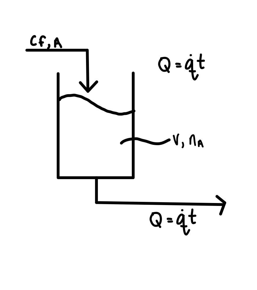
\end{align} y ( x ) F = F 1 ( ∫ F r d x + c ) = exp ( ∫ p d x ) Example: Mole balance on a tank with increasing inlet/outlet flow rate ¶ A stream with concentration c f , A c_{{\rm f},{\rm A}} c f , A V at a continuously increasing volumetric flow rate
Q = q ˙ t Q = \dot q t Q = q ˙ t q ˙ \dot q q ˙ t is time. A well-mixed stream is withdrawn from the tank at the same rate.
If there are initial n A , 0 n_{{\rm A},0} n A , 0 n A n_{\rm A} n A
Formulate overall mole balances based on entering and exit streams.
d n A d t = n ˙ A , i n − n ˙ A , o u t \dd{}{n_{\rm A}}{t} = \dot{n}_{{\rm A},\rm{in}} - \dot{n}_{{\rm A},\rm{out}} d t d n A = n ˙ A , in − n ˙ A , out Replace the molar flowrates with the equivalent concentrations and volumetric
flow rates
n ˙ A , i n = c f , A Q = c f , A q ˙ t n ˙ A , o u t = n A V Q = n A V q ˙ \begin{align}
\dot{n}_{{\rm A},\rm{in}} &= c_{{\rm f},{\rm A}} Q =
c_{{\rm f},{\rm A}} \dot{q}t \\
\dot{n}_{{\rm A},\rm{out}} &= \frac{n_{\rm A}}{V} Q =
\frac{n_{\rm A}}{V} \dot{q}
\end{align} n ˙ A , in n ˙ A , out = c f , A Q = c f , A q ˙ t = V n A Q = V n A q ˙ so the initial value problem is
n ˙ A = c f , A q ˙ t − n A V q ˙ t , n A ( 0 ) = n A , 0 \dot{n}_{\rm A} = c_{{\rm f},{\rm A}}\dot{q}t - \frac{n_{\rm A}}{V} \dot{q}t,
\quad n_{\rm A}(0) = n_{{\rm A},0} n ˙ A = c f , A q ˙ t − V n A q ˙ t , n A ( 0 ) = n A , 0 Rewrite in standard form
n ˙ A + ( q ˙ t V ) n A = c f , A q ˙ t \dot{n}_{A} + \left(\frac{\dot{q}t}{V}\right) n_{\rm A} = c_{{\rm f},{\rm A}} \dot{q}t n ˙ A + ( V q ˙ t ) n A = c f , A q ˙ t This is a linear first-order ODE with
p = q ˙ t V r = c f , A q ˙ t p = \frac{\dot{q}t}{V} \qquad r = c_{{\rm f},{\rm A}} \dot{q}t p = V q ˙ t r = c f , A q ˙ t that can be solved using an integrating factor:
F = e ∫ p d t = exp ( ∫ q ˙ t V d t ) = exp ( 1 2 q ˙ t 2 V ) F = e^{\int p \d{t}} = \exp\left(\int{\frac{\dot{q}t}{V} \d{t}}\right) =
\exp\left(\frac{1}{2}\frac{\dot{q} t^2}{V}\right) F = e ∫ p d t = exp ( ∫ V q ˙ t d t ) = exp ( 2 1 V q ˙ t 2 ) Then, evaluate the integral
∫ F r d t = ∫ exp ( 1 2 q ˙ t 2 V ) c f , A q ˙ t d t = ∫ e u c f , A V d u = c f , A V e u = c f , A V exp ( 1 2 q ˙ t 2 V ) \begin{align}
\int F r \d{t} &= \int \exp\left(\frac{1}{2}\frac{\dot{q} t^2}{V}\right)
c_{{\rm f},{\rm A}}\dot{q}t \d{t} \\
&= \int{e^{u}c_{{\rm f},{\rm A}}Vdu} \\
&= c_{{\rm f},{\rm A}}V e^u \\
&= c_{{\rm f},{\rm A}}V \exp\left(\frac{1}{2}\frac{\dot{q}t^2}{V}\right)
\end{align} ∫ F r d t = ∫ exp ( 2 1 V q ˙ t 2 ) c f , A q ˙ t d t = ∫ e u c f , A V d u = c f , A V e u = c f , A V exp ( 2 1 V q ˙ t 2 ) using the u substitution:
u = 1 2 q ˙ t 2 V d u = q ˙ t V d t \begin{align}
u &= \frac{1}{2}\frac{\dot{q} t^2}{V} \\
\d{u} &= \frac{\dot{q} t}{V} \d{t}
\end{align} u d u = 2 1 V q ˙ t 2 = V q ˙ t d t Last, combine the results:
n A ( t ) = 1 F ( ∫ F r d t + c ) = c f , A V + c exp ( − 1 2 q ˙ t 2 V ) \begin{align}
n_{\rm A}(t) &= \frac{1}{F} \left(\int F r \d{t} + c \right) \\
&= c_{{\rm f},{\rm A}} V + c \exp\left(-\frac{1}{2}\frac{\dot{q}t^2}{V}\right)
\end{align} n A ( t ) = F 1 ( ∫ F r d t + c ) = c f , A V + c exp ( − 2 1 V q ˙ t 2 ) Use the inital conditions to evaluate the integration constant:
n A ( 0 ) = c f , A V + c = n A , 0 c = n A , 0 − c f , A V \begin{align}
n_{\rm A}(0) &= c_{{\rm f},{\rm A}}V + c = n_{{\rm A},0} \\
c &= n_{{\rm A}, 0} - c_{{\rm f},{\rm A}} V
\end{align} n A ( 0 ) c = c f , A V + c = n A , 0 = n A , 0 − c f , A V The final result is:
n A ( t ) = c f , A V + ( n A , 0 − c f , A V ) exp ( − 1 2 q ˙ t 2 V ) n_{\rm A}(t) = c_{{\rm f},{\rm A}}V + (n_{{\rm A},0} - c_{{\rm f},{\rm A}}V) \exp\left(-\frac{1}{2}\frac{\dot{q}t^2}{V}\right) n A ( t ) = c f , A V + ( n A , 0 − c f , A V ) exp ( − 2 1 V q ˙ t 2 ) Example: Hormone level (again) ¶ We had
c ′ + k c = A + B cos ( π t 12 ) , c ( 0 ) = c 0 c' + kc = A + B\cos\left(\frac{\pi t}{12}\right), \quad c(0) = c_0 c ′ + k c = A + B cos ( 12 π t ) , c ( 0 ) = c 0 This is a linear first-order ODE with:
p = k c r = A + B cos ( π t 12 ) p = kc \qquad r = A + B\cos\left(\frac{\pi t}{12}\right) p = k c r = A + B cos ( 12 π t ) that can be solved using an integrating factor:
F = e ∫ k d t = e k t F = e^{\int k \d{t}} = e^{kt} F = e ∫ k d t = e k t Then, evaluate the integral using the table of integrals or integration by parts
to evaluate the second integral in the equation
∫ F r d t = ∫ e k t [ A + B cos ( π t 12 ) ] d t = A ∫ e k t d t + B ∫ e k t cos ( π t 12 ) d t = A k e k t + B e k t k 2 + ( π / 12 ) 2 [ k cos ( π t 12 ) + π 12 sin ( π t 12 ) ] \begin{align}
\int F r \d{t} &= \int e^{kt}
\left[A+B\cos\left(\frac{\pi t}{12}\right)\right]\d{t} \\
&= A\int e^{kt} \d{t} + B \int e^{kt} \cos\left(\frac{\pi t}{12}\right)\d{t} \\
&= \frac{A}{k} e^{kt} + B \frac{e^{kt}}{k^{2}+(\pi/12)^2}
\Biggl[k \cos{(\frac{\pi t}{12})} +
\frac{\pi}{12}\sin{\left(\frac{\pi t}{12}\right)}\Biggr]
\end{align} ∫ F r d t = ∫ e k t [ A + B cos ( 12 π t ) ] d t = A ∫ e k t d t + B ∫ e k t cos ( 12 π t ) d t = k A e k t + B k 2 + ( π /12 ) 2 e k t [ k cos ( 12 π t ) + 12 π sin ( 12 π t ) ] The general solution is:
c ( t ) = 1 F ( ∫ F r d t + c ∗ ) = A k + B k 2 + ( π / 12 ) 2 [ k cos ( π t 12 ) + π 12 sin ( π t 12 ) ] + c ∗ e − k t \begin{align}
c(t) &= \frac{1}{F} \left(\int F r \d{t} + c^* \right) \\
&= \frac{A}{k} + \frac{B}{k^{2}+(\pi/12)^2}
\Biggl[k \cos\left(\frac{\pi t}{12}\right)
+ \frac{\pi}{12}\sin{\left(\frac{\pi t}{12}\right)}\Biggr] +
c^* e^{-kt}
\end{align} c ( t ) = F 1 ( ∫ F r d t + c ∗ ) = k A + k 2 + ( π /12 ) 2 B [ k cos ( 12 π t ) + 12 π sin ( 12 π t ) ] + c ∗ e − k t Use the inital condition to evaluate the integration constant:
c ( 0 ) = A k + B k 2 + ( π / 12 ) 2 k + c ∗ = c 0 c ∗ = c 0 − A k − B k 2 + ( π / 12 ) 2 k \begin{align}
c(0) &= \frac{A}{k} + \frac{B}{k^{2}+(\pi/12)^2} k + c^* = c_0 \\
c^* &= c_0 - \frac{A}{k} - \frac{B}{k^{2}+(\pi/12)^2} k
\end{align} c ( 0 ) c ∗ = k A + k 2 + ( π /12 ) 2 B k + c ∗ = c 0 = c 0 − k A − k 2 + ( π /12 ) 2 B k The final solution is:
c ( t ) = A k + B k 2 + ( π / 12 ) 2 [ k cos ( π t 12 ) + π 12 sin ( π t 12 ) ] + [ c 0 − A k − B k k 2 + ( π / 12 ) 2 ] e − k t \begin{align}
c(t) &= \frac{A}{k} +
\frac{B}{k^{2}+(\pi/12)^2} \Biggl[k \cos\left(\frac{\pi t}{12}\right) +
\frac{\pi}{12}\sin{\left(\frac{\pi t}{12}\right)}\Biggr] \\
&+ \Biggl[c_0 - \frac{A}{k} - \frac{Bk}{k^{2}+(\pi/12)^2} \Biggr] e^{-kt}
\end{align} c ( t ) = k A + k 2 + ( π /12 ) 2 B [ k cos ( 12 π t ) + 12 π sin ( 12 π t ) ] + [ c 0 − k A − k 2 + ( π /12 ) 2 B k ] e − k t Skill builder problems ¶ Solve the following differential equations:
This ODE is not in the standard form, so we need to first rearrange:
x y d y = ( x 4 + y 2 ) d x ( x 4 + y 2 ) d x − x y d y = 0 \begin{align}
xy \d{y} = (x^4+y^2) \d{x} \\
(x^4 + y^2) \d{x} - xy \d{y} = 0
\end{align} x y d y = ( x 4 + y 2 ) d x ( x 4 + y 2 ) d x − x y d y = 0 so:
P = x 4 + y 2 Q = − x y \begin{align}
P &= x^4 + y^2 \\
Q &= -xy
\end{align} P Q = x 4 + y 2 = − x y Check to see if the ODE is exact:
( ∂ P ∂ y ) x = 2 y ( ∂ Q ∂ x ) y = − y \begin{align}
\td{}{P}{y}{x} &= 2y \\
\td{}{Q}{x}{y} &= -y
\end{align} ( ∂ y ∂ P ) x ( ∂ x ∂ Q ) y = 2 y = − y The two partial derivatives are not equal, so the ODE is not exact. In
order to make it exact, we need to find an integrating factor F . First,
compute:
R = 1 Q [ ( ∂ P ∂ y ) x − ( ∂ Q ∂ x ) y ] = 1 − x y ( 2 y − ( − y ) ) = − 3 x \begin{align}
R &= \frac{1}{Q}\left[\td{}{P}{y}{x} - \td{}{Q}{x}{y} \right] \\
&=\frac{1}{-xy}(2y-(-y)) \\
&= -\frac{3}{x}
\end{align} R = Q 1 [ ( ∂ y ∂ P ) x − ( ∂ x ∂ Q ) y ] = − x y 1 ( 2 y − ( − y )) = − x 3 R is a function of only x , so use it to compute F
F = exp ( ∫ − 3 x d x ) = e − 3 ln ( x ) = x − 3 F = \exp\left(\int \frac{-3}{x} \d{x}\right) = e^{-3\ln(x)} = x^{-3} F = exp ( ∫ x − 3 d x ) = e − 3 l n ( x ) = x − 3 Apply the integrating factor to the original ODE:
x − 3 ( x 4 + y 2 ) d x − x − 3 ( x y ) d y = 0 ( x + y 2 x − 3 ) d x − y x 2 d y = 0 \begin{align}
x^{-3}(x^4+y^2) \d{x} - x^{-3}(xy) \d{y} &= 0 \\
\left(x+\frac{y^2}{x^{-3}}\right) \d{x} - \frac{y}{x^2} \d{y} &= 0
\end{align} x − 3 ( x 4 + y 2 ) d x − x − 3 ( x y ) d y ( x + x − 3 y 2 ) d x − x 2 y d y = 0 = 0 Integrate the Q of our exact ODE with respect to y :
f ( x , y ) = ∫ − y x 2 d y = − y 2 2 x 2 + k ( x ) f(x,y) = \int -\frac{y}{x^2} \d{y} = \frac{-y^2}{2x^2}+k(x) f ( x , y ) = ∫ − x 2 y d y = 2 x 2 − y 2 + k ( x ) where k is an unknown function of x . Then, differentiate f with respect
to x and compare to P of the exact ODE:
( ∂ f ∂ x ) y = y 2 x 3 + k ′ ( x ) = P = x + y 2 x 3 k ′ ( x ) = x \begin{align}
\td{}{f}{x}{y} = \frac{y^2}{x^3} + k'(x) &= P = x + \frac{y^2}{x^3} \\
k'(x) &= x \\
\end{align} ( ∂ x ∂ f ) y = x 3 y 2 + k ′ ( x ) k ′ ( x ) = P = x + x 3 y 2 = x This ODE for k can be integrated directly (neglecting the integration
constant)
k = ∫ x d x = x 2 2 k = \int x \d{x} = \frac{x^2}{2} k = ∫ x d x = 2 x 2 Putting it all together,
f = − y 2 2 x 2 + x 2 2 = c \begin{align}
f = \frac{-y^2}{2x^2} + \frac{x^2}{2} = c
\end{align} f = 2 x 2 − y 2 + 2 x 2 = c is an implicit solution of the ODE.
This ODE is not in the standard form, so we need to first rearrange:
( e x + y + y e y ) d x + ( x e y − 1 ) d y = 0 \begin{align}
(e^{x+y} + ye^y) \d{x} + (x e^y - 1) \d{y} = 0
\end{align} ( e x + y + y e y ) d x + ( x e y − 1 ) d y = 0 so
P = e x + y + y e y Q = x e y − 1 \begin{align}
P &= e^{x+y} + ye^y \\
Q &= x e^y - 1
\end{align} P Q = e x + y + y e y = x e y − 1 Check if the differential equation is exact:
( ∂ P ∂ y ) x = e x + y + y e y + e y ( ∂ Q ∂ x ) y = e y \begin{align}
\td{}{P}{y}{x} &= e^{x+y} + y e^y + e^y \\
\td{}{Q}{x}{y} &= e^y
\end{align} ( ∂ y ∂ P ) x ( ∂ x ∂ Q ) y = e x + y + y e y + e y = e y These are not equal, so the equation is not exact. To make it exact, find
integrating factor F . The R formula gives:
R = 1 Q [ ( ∂ P ∂ y ) x − ( ∂ Q ∂ x ) y ] = 1 x e y − 1 ( e x + y + y e y + e y − e y ) = e y ( e x + y ) x e y − 1 \begin{align}
R &= \frac{1}{Q}\left[\td{}{P}{y}{x} - \td{}{Q}{x}{y} \right] \\
&=\frac{1}{x e^y - 1}(e^{x+y} + y e^y + e^y - e^y) \\
&= \frac{e^y(e^x + y)}{x e^y - 1}
\end{align} R = Q 1 [ ( ∂ y ∂ P ) x − ( ∂ x ∂ Q ) y ] = x e y − 1 1 ( e x + y + y e y + e y − e y ) = x e y − 1 e y ( e x + y ) this is not a function of only x , so try the S formula:
S = − Q P R = − e y ( e x + y ) e x + y + y e y = − 1 \begin{align}
S &= -\frac{Q}{P} R \\
&= -\frac{e^y(e^x + y)}{e^{x+y} + y e^y} \\
&= -1
\end{align} S = − P Q R = − e x + y + y e y e y ( e x + y ) = − 1 This is a function of, at most, y so:
F = exp ( ∫ S d y ) = e − y F = \exp\left(\int S\d{y} \right) = e^{-y} F = exp ( ∫ S d y ) = e − y Multiply the equation by F :
( e x + y ) d x + ( x − e − y ) d y = 0 (e^x + y) \d{x} + (x - e^{-y}) \d{y} = 0 ( e x + y ) d x + ( x − e − y ) d y = 0 Now the equation is exact so integrate the new P with respect to x :
f ( x , y ) = ∫ ( e x + y ) d x = e x + x y + k ( y ) f(x,y) = \int (e^x + y) \d{x} = e^x + xy + k(y) f ( x , y ) = ∫ ( e x + y ) d x = e x + x y + k ( y ) where k is an unknown function of y . Then, differentiate f with respect
to y and compare to Q :
( ∂ f ∂ x ) y = x + k ′ ( y ) = Q = x − e − y k ′ = − e − y \begin{align}
\td{}{f}{x}{y} = x + k'(y) &= Q = x - e^{-y} \\
k' &= -e^{-y}
\end{align} ( ∂ x ∂ f ) y = x + k ′ ( y ) k ′ = Q = x − e − y = − e − y This ODE for k can be integrated directly (neglecting the integration constant)
k ( y ) = ∫ − e − y d y = e − y \begin{align}
k(y) = \int -e^{-y} \d{y} = e^{-y}
\end{align} k ( y ) = ∫ − e − y d y = e − y Putting it all together,
f ( x , y ) = e x + e − y + x y = c \begin{align}
f(x, y) = e^x + e^{-y} + xy = c
\end{align} f ( x , y ) = e x + e − y + x y = c is an implicit solution for the ODE.
Rewrite in linear form:
y ′ − y = 1 − 2 x \begin{align}
y' - y = 1 - 2x
\end{align} y ′ − y = 1 − 2 x where
p = − 1 r = 1 − 2 x \begin{align}
p = -1 \qquad r = 1 - 2x
\end{align} p = − 1 r = 1 − 2 x Find integrating factor:
F = e ∫ p d x = e ∫ − 1 d x = e − x \begin{align}
F = e^{\int p\d{x}} = e^{\int -1 \d{x}} = e^{-x}
\end{align} F = e ∫ p d x = e ∫ − 1 d x = e − x Then, evaluate the integral
∫ F r d x = ∫ e − x ( 1 − 2 x ) d x \int F r \d{x} = \int e^{-x} (1-2x) \d{x} ∫ F r d x = ∫ e − x ( 1 − 2 x ) d x This integral can be evaluated by parts using the tabular method:
sign u u u d v \d{v} d v e − x e^{-x} e − x + + + 1 − 2 x 1-2x 1 − 2 x − e − x -e^{-x} − e − x − - − -2 e − x e^{-x} e − x 0
so
∫ F r d x = ( 2 x − 1 ) e − x + 2 e − x = ( 2 x + 1 ) e − x \int F r \d{x} = (2x-1)e^{-x} + 2 e^{-x} = (2x + 1) e^{-x} ∫ F r d x = ( 2 x − 1 ) e − x + 2 e − x = ( 2 x + 1 ) e − x Putting it all together:
y = 1 F ( ∫ F r d x + c ) = e x [ ( 2 x + 1 ) e − x + c ] = 1 + 2 x + c e x \begin{align}
y &= \frac{1}{F}\left(\int F r \d{x} + c \right) \\
&= e^x \left[ (2x + 1) e^{-x} + c \right] \\
&= 1 + 2x + c e^x
\end{align} y = F 1 ( ∫ F r d x + c ) = e x [ ( 2 x + 1 ) e − x + c ] = 1 + 2 x + c e x