3.3. Gauss–Jordan elimination#
Example: Pump circuit
Incompressible flow can be written analogous to an electrical circuit as
where \(\Delta P\) is the pressure change, R is the resistance, and Q is the volumetric flow rate. For the following pump “circuit”:
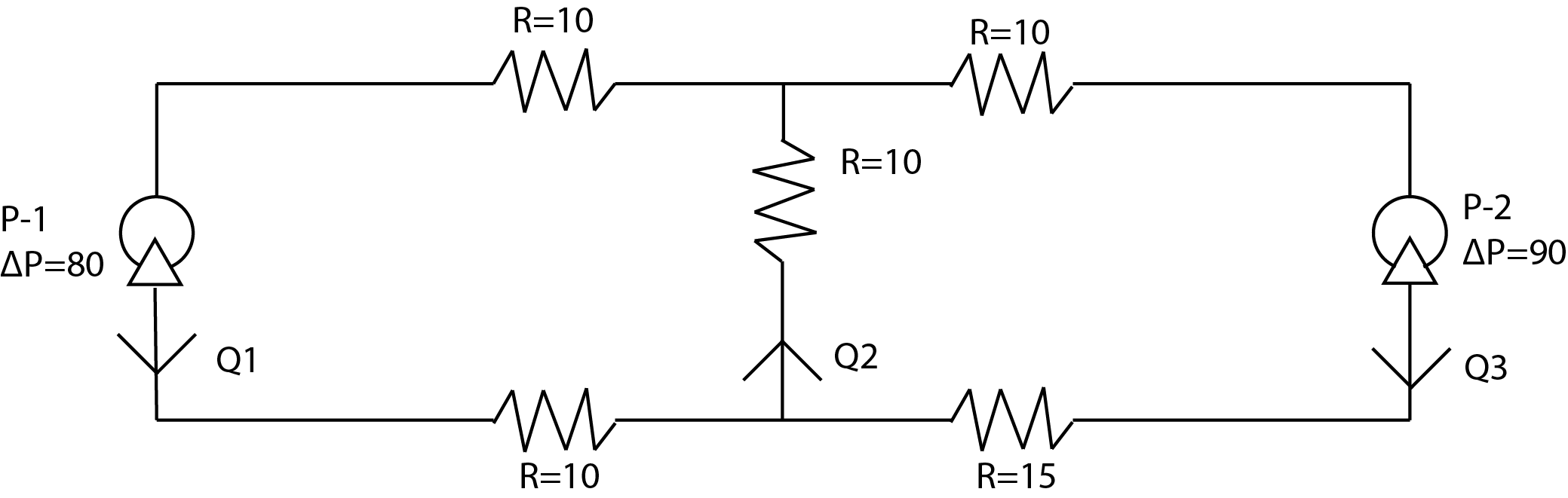
The pressure and mass balances for the nodes and loop give:
Find \(Q_1\), \(Q_2\), and \(Q_3\).
First, rearrange the equations into consistent linear form:
Then, rewrite using matrix representation:
Now, perform Gauss-Jordan elimination steps to solve for the unknown flow rates. We form the augmented matrix, then use Row 1 to eliminate values in Rows 2 and 3:
Row 2 is all zeros because it was a redundant equation to Row 1. Swap Rows 2 and 4, then use the new Row 2 to eliminate value in Row 3:
Normalize Row 3 (divide by -95), then eliminate values above in Column 3:
Normalize Row 2 (divide by 10), then eliminate values above in Column 2:
Turning back into an equivalent system of equations gives the final solution, \(Q_1 = 2\), \(Q_2 = 4\), and \(Q_3 = 2\).
3.3.1. Skill builder problems#
Solve using Gauss-Jordan elimination
(3.35)#\[\begin{align} 5 x_1 - 2 x_2 &= 20.9 \\ -x_1 + 4x_2 &= -19.3 \end{align}\]Solution
Form the augmented matrix and perform row reduction:
(3.36)#\[\begin{align} \begin{bmatrix} 5 & -2 & 20.9 \\ -1 & 4 & -19.3 \end{bmatrix} \begin{matrix} {\rm swap} \\ \vphantom{R_2}\end{matrix} &\to \begin{bmatrix} -1 & 4 & -19.3 \\ 5 & -2 & 20.9\end{bmatrix} \begin{matrix} \times -1 \\ \vphantom{R_2}\end{matrix} \\ &\to \begin{bmatrix} 1 & -4 & 19.3 \\ 5 & -2 & 20.9\end{bmatrix} \begin{matrix} \vphantom{R_1} \\ -5 R_1 \end{matrix} \\ &\to \begin{bmatrix} 1 & -4 & 19.3 \\ 0 & 18 & -75.6\end{bmatrix} \begin{matrix} \vphantom{R_1} \\ \div 18 \end{matrix} \\ &\to \begin{bmatrix} 1 & -4 & 19.3 \\ 0 & 1 & -4.2\end{bmatrix} \begin{matrix} +4 R_2 \\ \vphantom{R_2} \end{matrix} \\ &\to \begin{bmatrix} 1 & 0 & 2.5 \\ 0 & 1 & -4.2\end{bmatrix} \end{align}\]so \(x_1 = 2.5\) and \(x_2 = -4.2\).
Solve using Gauss-Jordan elimination
(3.37)#\[\begin{align} x_1 + 4 x_2 = 8 \\ 2 x_1 + 8 x_2 = 17 \end{align}\]Solution
(3.38)#\[\begin{align} \begin{bmatrix} 1 & 4 & 8 \\ 2 & 8 & 17 \end{bmatrix} \begin{matrix} \vphantom{R_1} \\ -2 R_1\end{matrix} &\to \begin{bmatrix} 1 & 4 & 8 \\ 0 & 0 & 1\end{bmatrix} \end{align}\]The equations do not have a solution because the last row is false.
Solve using Gauss-Jordan elimination
(3.39)#\[\begin{align} x_1 + x_2 + x_2 = 2 \\ 4x_2 + 6 x_3 = -12 \\ x_1 + x_2 + x_3 = 2 \end{align}\]Solution
(3.40)#\[\begin{align} \begin{bmatrix} 0 & 1 & 1 & -2 \\ 0 & 4 & 6 & -12 \\ 1 & 1 & 1 & 2 \end{bmatrix} \begin{matrix} \vphantom{R_1} \\ \rm shuffle \\ \vphantom{R_3} \end{matrix} &\to \begin{bmatrix} 1 & 1 & 1 & 2 \\ 0 & 1 & 1 & -2 \\ 0 & 4 & 6 & -12 \end{bmatrix} \begin{matrix} \vphantom{R_1} \\ \vphantom{R_2} \\ \ -4 R_2 \end{matrix} \\ &\to \begin{bmatrix} 1 & 1 & 1 & 2 \\ 0 & 1 & 1 & -2 \\ 0 & 0 & 2 & -4 \end{bmatrix} \begin{matrix} \vphantom{R_1} \\ \vphantom{R_2} \\ \div 2 \end{matrix} \\ &\to \begin{bmatrix} 1 & 1 & 1 & 2 \\ 0 & 1 & 1 & -2 \\ 0 & 0 & 1 & -2 \end{bmatrix} \begin{matrix} -R_3 \\ -R_3 \\ \vphantom{R_3} \end{matrix} \\ &\to \begin{bmatrix} 1 & 1 & 0 & 4 \\ 0 & 1 & 0 & 0 \\ 0 & 0 & 1 & -2 \end{bmatrix} \begin{matrix} -R_2 \\ \vphantom{R_2} \\ \vphantom{R_3} \end{matrix} \\ &\to \begin{bmatrix} 1 & 0 & 0 & 4 \\ 0 & 1 & 0 & 0 \\ 0 & 0 & 1 & -2 \end{bmatrix} \end{align}\]so \(x_1 = 4\), \(x_2 = 0\), and \(x_3 = -2\).