Example: Pump circuit
Incompressible flow can be written analogous to an electrical circuit as
(3.27)\[\begin{equation}
-\Delta P = RQ
\end{equation}\]
where \(\Delta P\) is the pressure change, R is the resistance, and Q is the
volumetric flow rate. For the following pump “circuit”:
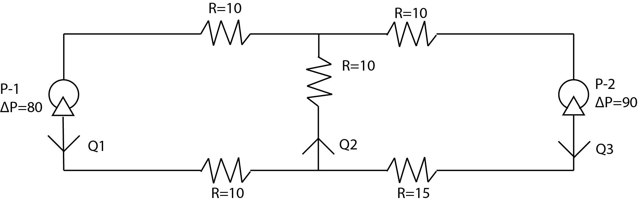
The pressure and mass balances for the nodes and loop give:
(3.28)\[\begin{align}
Q_1 &+ Q_3 = Q_2 \\
Q_2 &= Q_1 + Q_3 \\
80 &= 10Q_2 + 20Q_1 \\
90 &= 25Q_3 + 10Q_2
\end{align}\]
Find \(Q_1\), \(Q_2\), and \(Q_3\).
First, rearrange the equations into consistent linear form:
(3.29)\[\begin{align}
Q_1 - Q_2 + Q_3 &= 0 \\
Q_1 - Q_2 + Q_3 &= 0 \\
20Q_1 + 10Q_2 + 0Q_3 &= 80 \\
0Q_1 + 10Q_2 + 25Q_3 &= 90
\end{align}\]
Then, rewrite using matrix representation:
(3.30)\[\begin{equation}
\begin{bmatrix}
1 & -1 & 1 \\
1 & -1 & 1 \\
20 & 10 & 0 \\
0 & 10 & 25
\end{bmatrix}
\begin{bmatrix}
Q_1 \\ Q_2 \\ Q_3
\end{bmatrix}
= \begin{bmatrix}
0 \\ 0 \\ 80 \\ 90
\end{bmatrix}
\end{equation}\]
Now, perform Gauss-Jordan elimination steps to solve for the unknown flow rates.
We form the augmented matrix, then use Row 1 to eliminate values in Rows 2 and
3:
(3.31)\[\begin{equation}
\begin{bmatrix}
1 & -1 & 1 & 0 \\
-1 & 1 & -1 & 0 \\
20 & 10 & 0 & 80 \\
0 & 10 & 25 & 90
\end{bmatrix}
\begin{matrix}
\vphantom{R_1} \\ + R_1 \\ -20 R_1 \\ \vphantom{R_1}
\end{matrix}
\to
\begin{bmatrix}
1 & -1 & 1 & 0 \\
0 & 0 & 0 & 0 \\
0 & 30 & -20 & 80 \\
0 & 10 & 25 & 90
\end{bmatrix}
\end{equation}\]
Row 2 is all zeros because it was a redundant equation to Row 1. Swap Rows 2 and
4, then use the new Row 2 to eliminate value in Row 3:
(3.32)\[\begin{equation}
\begin{bmatrix}
1 & -1 & 1 & 0 \\
0 & 10 & 25 & 90 \\
0 & 30 & -20 & 80 \\
0 & 0 & 0 & 0
\end{bmatrix}
\begin{matrix}
\vphantom{R_1} \\ \vphantom{R_1} \\ -3 R_2 \\ \vphantom{R_1}
\end{matrix}
\to \begin{bmatrix}
1 & -1 & 1 & 0 \\
0 & 10 & 25 & 90 \\
0 & 0 & -95 & -190 \\
0 & 0 & 0 & 0
\end{bmatrix}
\end{equation}\]
Normalize Row 3 (divide by -95), then eliminate values above in Column 3:
(3.33)\[\begin{equation}
\begin{bmatrix}
1 & -1 & 1 & 0 \\
0 & 10 & 25 & 90 \\
0 & 0 & 1 & 2 \\
0 & 0 & 0 & 0
\end{bmatrix}
\begin{matrix}
- R_3 \\ -25 R_3 \\ \vphantom{R_1} \\ \vphantom{R_1}
\end{matrix}
\to
\begin{bmatrix}
1 & -1 & 0 & -2 \\
0 & 10 & 0 & 40 \\
0 & 0 & 1 & 2 \\
0 & 0 & 0 & 0
\end{bmatrix}
\end{equation}\]
Normalize Row 2 (divide by 10), then eliminate values above in Column 2:
(3.34)\[\begin{equation}
\begin{bmatrix}
1 & -1 & 0 & -2 \\
0 & 1 & 0 & 4 \\
0 & 0 & 1 & 2 \\
0 & 0 & 0 & 0
\end{bmatrix}
\begin{matrix}
+ R_2 \\ \vphantom{R_1} \\ \vphantom{R_1} \\ \vphantom{R_1}
\end{matrix}
\to
\begin{bmatrix}
1 & 0 & 0 & 2 \\
0 & 1 & 0 & 4 \\
0 & 0 & 1 & 2 \\
0 & 0 & 0 & 0
\end{bmatrix}
\end{equation}\]
Turning back into an equivalent system of equations gives the final solution,
\(Q_1 = 2\), \(Q_2 = 4\), and \(Q_3 = 2\).